Energy Based Models Part 3: Generative AI Using EBMs
Contents
- Introduction
- EBMs with ANN based Energy Functions
- Using EBMs to Generate Images
- Text to Image Generation
- Generative EBMs as Models for Biological Brains
- MCMC Sampling Using Langevin Dynamics
- Training EBMS Using Score Functions
- Noise Conditional Score Networks (NCSN)
- Training EBMS Using Maximum Likelihood Algorithm
- The Diffusion Recovery Likelihood (DRL) Algorithm
- Hardware Implementation of EBMs
Abstract
Modern generative artificial neural networks such as LLMs show signs of human like intelligence. Can their operation be tied back to principles of physics, in particular thermodynamics? If so, it will provide a plausible picture of how the brain works, since it too presumably functions using natural laws. In this article we will discuss how Energy Based Models (EBMs) can be made to function as generative models, which brings us one step closer in this quest.
When I started writing this series of articles, the initial system that I described was the Ising model for magnetism, and how phase changes in the material could be used to explain its properties. We looked at other models with more complex node interactions called spin glasses, and this led to the discovery that they also exhibit phases, but they have many more phases compared to magnets. In the present article we will see that the process of generating images can be considered to be type of phase change created by the interactions of hundreds of thousands of individual nodes of the spin glass type interacting with each other. But the law that governs these phases is the same one that we encountered when studying magnetism, which is to say the principle of minimization of energy, and here is a high level description:
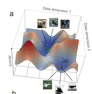
Figure 1: The energy landscape in an image generation EBM
- Assuming that there are $N$ nodes $X=(x_1,…,x_N)$ in a generative EBM used to generate images, such that $X$ corresponds to an image and $x_i$ is the $i^{th}$ pixel value. The energy for this system is modeled by a function $E_W(x_1,…,x_N)$, where $W$ represents its learnable parameters. Once the model has been trained, images are arranged in the landscape of this energy function, in which the bottom of valleys corresponds to images that are similar to those in the training set (see figure 1).
- The process of generation consists of starting from an initial state in the state space (which may look like noise to us), and then traversing the energy landscape until the system arrives at a minima, and at this point the configuration looks like an intelligible image.
If you recall the design of Boltzmann machines in Part 2, the above description looks very similar, but there are a few differences.
- The state space in a Boltzmann machine is made up of binaries 1 or 0, while in modern EBMs it can be a real number $x$.
- Boltzmann machines feature a simple quadratic energy function, whereas in modern EBMs it can be an arbitrarily complex function $E_W(x_1,…,x_N)$.
- Generation is done by sampling in both cases, however the Gibbs sampling used in Boltzmann machines cannot be used if the energy function does not have the quadratic form. Instead a more powerful sampling algorithm, namely Langevin sampling, is used.
In all likelihood biological brains operate using thermodynamic principles and it is not inconceivable that their architecture and that of generative EBMs share common principles of operation since the same physics underlies both (this is not unlike the fact that both birds and airplanes are able to fly using the Bernoulli’s principle from physics, but they use different mechanisms). However brains are architected very differently compared to modern artificial neural networks (ANNS) such as the transformer, in particular they have an extensive amount of feedback connections. In contrast, transformers use a feed-forward type architecture, and this is also true for other ANNs such convolutional neural networks or CNNs. The EBM approach to generative modeling gets around this conundrum by proposing that the transformer could be a model for the energy function of the brains neural network, rather than for its inter-connection topology. This bypasses the problem of figuring out the interconnection architecture of biological brains, in which there has been limited progress, and shifts the focus to the principle of minimization of the energy function, which is based on thermodynamics, and underlies the operation of both brains and EBM models.
The EBM approach to generative modeling also provides insight into the question of how brains are able to operate using much lower energy compared to LLMs. The parallelism in modern ANNs is a good match for implementation on GPUs, which are responsible for all that energy consumption. The basic operation in EBMs on the other hand is sampling which is not a good fit for GPUs. However the sampling operation can be made much more efficient by exploiting the physical properties of the substrate on which the system is built, and this is presumably what our brains are doing. Towards the end of the article I will describe some efforts underway to create devices that are able to sample in an energy efficient manner.
Introduction
The process of generation, whether images or text, is based on the idea of sampling from a probability distribution that approximates the statistics of the training data. Hinton and Sejnowski were the first ones to realize the power of this idea, and showed how to obtain an EBM model for the probability distribution by choosing the interaction strengths in a Sherrington-Kirkpatrick type spin glass model, that they called a Boltzmann machine. These systems worked well, but failed to scale up and also suffered from long convergence times. So the question arises whether we can improve on the Boltzmann machine and create a modern EBM that can scale to hundreds of thousands of nodes, with performance that is comparable to non-EBM artificial neural networks (ANN) models. We have made a good deal of progress in the last decade or so towards this goal, and this is described in this article.
Boltzmann machine based EBM models entered a winter phase following the success of feed-forward type ANNs, heralded by the AlexNet model of 2012 (which also came out of Hinton’s research group), and more recently with the transformer based LLM models from Google, OpenAI and others. However beginning in 2019 there has been a renewed interest in EBMs, led by research coming from academia, such as by Stefano Ermon’s group at Stanford University, which has led to considerable progress in the modeling capability of EBMs.
The original Boltzmann machines never became commercially viable due to a couple of problems:
- They were not able to scale up to beyond a few hundred nodes since the training process became too time consuming. This was due to the fact that the sampling algorithm was not able to handle multi-model distributions very well. It took an excessive amount of time to move between valleys in the energy landscape during the sampling process.
- It was limited to the quadratic energy function with per node state values of 0 and 1 (or -1 and 1). In order to compete with ANNs there was a need to extend it to more general energy functions and node values that are real numbers.
Modern generative EBMs are also based on the idea of approximating the training data distribution $p(x_1,…,x_N)$ by a Boltzmann distribution $p_W(x_1,…,x_N)$ and then sampling from it. Recall that if $E_W$ is the energy function for the model, then its Boltzmann distribution can be written as
\[p_W(x_1,...,x_N) = {e^{-E_W(x_1,...,x_N)}\over{Z_W}}\]where $Z_W$ is the partition function, and in general getting an estimate for it is a challenging problem. Hinton’s original design for training the Boltzmann machine got around this by sampling from $p_W$, which can be done without knowing $Z_W$, but unfortunately this algorithm was not able to scale up. Modern EBMs solve this problem by borrowing an idea that was used in the simulated annealing algorithm, i.e., introducing noise into the system and then gradually reducing it as the sampling progresses.
It was also discovered recently that there is a way to sample from EBMs based on estimating the gradient of the energy function ${\partial E_W\over{\partial x_i}}$, also called the score function. This allows us to generate samples from the probability distribution $p_W(x_1,…,x_N)$ without knowing what its energy function $E_W$ is. This fundamental idea was discovered by several people around the turn of the millennium, and underlies a generative EBM model called Noise Conditioned Score Networks or NCSN.
In order to fully exploit these ideas, we also need to generalize beyond the quadratic energy functions used in Boltzmann machines. ANNs are well suited for this task, since they provide us with a way to to model arbitrarily complex functions. Thus the energy function $E_W(x_1,…,x_N)$ is now a neural network and the parameters $W$ of the ANN play the role of interaction strengths in the original Boltzmann machine. Using this idea it becomes possible to replace the quadratic energy function in the Boltzmann machine, with an ANN which can potentially have hundreds of thousands of parameters and this results in an enormous increase in the modeling power of the resulting EBM. This also enables modern EBMs to piggyback on the advances in ANNs in recent years with powerful models such as convolutional neural networks (CNNs) and transformers used to model $E_W$.
In order to design modern EBMs there are two problems that have to be solved:
- How to sample from these models since the Gibbs sampling used in classical Boltzmann machines only applies for quadratic energy functions.
- How to train these models, since Hinton’s algorithm for training the Boltzmann machines cannot be used anymore.
The first issue was resolved with the discovery of Langevin based Markov Chain Monte Carlo (MCMC) sampling. This algorithm can be used if we know the energy function $E_W$ or the score function ${\partial E_W\over{\partial x_i}}$ for the model. Furthermore the system state can be a real number (as opposed to binary numbers in the Boltzmann machine). The sampling operation causes the state to converge to values distributed according to a specified probability distribution which in this case is the Boltzmann distribution $p_W$. The origins of Langevin sampling lie in the theory of stochastic differential equations, and I touched upon this topic in my article on Brownian Motion. Once we use Langevin sampling, it becomes possible to handle energy functions that are more complex than quadratic, indeed it becomes possible use arbitrarily complex energy functions such as those modeled by CNNs and transformers.
There also has been progress in training algorithms for EBMs. Hinton’s original algorithm for training Boltzmann Machines was based on the concept of maximizing the likelihood function for the training data (or equivalently minimizing the KL divergence between the training data distribution and the model provided distribution). This solution was based on Gibbs sampling and led to excessive convergence times. The resolution to this problem required some fundamental advances in theory, and interestingly enough the core idea that finally solved it is related to the idea of simulated annealing that was described in Part 1. It was recognized that the problem had to do with the inefficient sampling of multi-modal distributions, and the solution involved mixing noise to the system state in order to make the distribution closer to unimodal. More important was the idea of introducing this noise at various levels of intensity and then gradually reducing it from high to low values during the sampling process. It was shown that this indeed solved the multi-modality problem and led to model outputs that are currently the state of the art in image generation. These models generally go by the name of diffusion models and can be considered to be the modern versions of the Boltzmann Machines with upgraded energy functions and training algorithms.
All these advances in EBM models are impressive, but is there any fundamental benefit to using them over non-EBM models since it seems that both types of models are equally good at various tasks? The current generation of non-EBM models are based on the backprop algorithm for training, and this can be considerably accelerated with the help of GPUs. However this comes with the problem of sky-rocketing energy consumption for large model sizes. If EBM models can be engineered for lower energy consumption then this would constitute a major benefit. If the sampling operation is implemented using analog components and can take advantage of the the physical properties of the hardware substrate on which these systems are built then it can potentially lead to huge savings in energy consumption. There are a number of efforts underway in this direction and we will describe a few of them towards the end of this article. These systems are still in the research phase and they have a long way to go until they can approach the performance of digitally implemented EBM systems.
The holy grail of modern generative systems are LLMs, and the question arises whether EBMs can be used to implement LLMs. The current generation of LLMs are based on auto-regressive sampling using transformers, and generate one word at a time. It turns out that that EBMs can also be used to generate language in a more holistic manner and there also has been progress in building reasoning models using EBMs. This topic is covered in Part 4, we will focus on image generation in this article.
There is another branch in modern EBM theory called Thermodynamic Computing which derives its inspiration from the original Hopfield network as opposed to the Boltzmann machine. Recall that the Hopfield network generated specific state configurations in equilibrium, as opposed to sampling from the distribution of the equilibrium configurations. This implies that it can potentially be used as a computational tool. This was actually pointed out by Hopfield himself, who showed how combinatorial optimization problems such as the Travelling Salesman Problem can be mapped on to and solved using the Hopfield network. This work has been updated by research groups at Purdue University and UCSB, who have shown how Hopfield networks can be scaled to much larger sizes, using both theoretical advances such as more efficient sampling techniques, as well new hardware devices that can implement this sampling more efficiently. This work is also in its research phase at the present time, and its main driver has been to serve as an alternative to quantum computers for implementing probabilistic algorithms.
EBMs with ANN Based Energy Functions
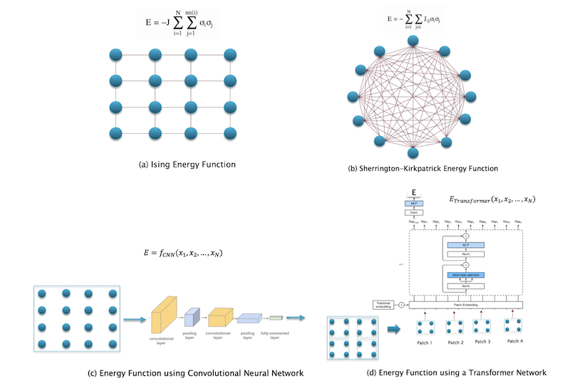
Figure 2: Computing the energy functions for EBMs
The original Ising model for magnetism featured a simple energy function, shown in part (a) of the above figure. The interaction strength between nodes was uniform across the entire network, and this resulted in an energy landscape with a couple of minima corresponding to net magnetization of the system. Sherrington and Kirkpatrick modified this model by making the interaction strengths random, and also allowed each node to interact with every other node in the system, shown in part (b). This led to a complex energy landscape with a large number of minima that scaled up with the number of nodes. The SK model was subsequently used by Hopfield and Hinton to create the first computational and generative models, namely the Hopfield network and the Boltzmann machine, as described in Part 2 of this article series.
A way for EBMs to transition to the modern era is shown in the lower part of the figure. Part (c) shows an energy function that is described by convolutional neural network or CNN which were originally introduced as a way to process images. Part (d) of the figure shows an EBM that uses the transformer network for computing energy functions. Transformers are a powerful way to model energy functions, traditional auto-regressive LLMs use them as a way to sample from conditional probability distributions. Note that neither of the EBMs in the lower part of the figure show inter-node interaction strengths, presumably these exist but are much more complex than the ones in the upper part of the figure. The focus has now shifted to modeling the energy function directly.
In the original EBMs shown in parts (a) and (b), the energy function was parametrized by the interaction strengths between nodes, on the other hand, if we use either a CNN or transformer (or any other ANN) to model the energy function, then the energy function is parametrized by the weights in the ANN. Indeed the modern theory of EBMs is based entirely on the energy functions, which can be as complex as we wish, as long as they can be represented by an artificial neural network. Since an ANN can be trained to approximate arbitrarily functions, it follows that these new EBMs is capable of modeling a much wider variety of energy landscapes.
Whether we use inter-node interactions or we use ANNs to model the energy function, in either case the probability of the system being in state $(x_1,x_2,…,x_N)$ is given by
\[p_W(x_1,x_2,...,x_N) = {e^{-E_W(x_1,...,x_N)}\over{Z_W}}\]where $Z_W$ as usual is the partition function
\[Z_W = \int_{x_1,...,x_N} e^{-E_W(x_1,...,x_N)} dx_1...dx_N\]Note that unlike the Boltzmann machine, the state variables $(x_1,…,x_N)$ are no longer restricted to $+1,-1$ but can take on any real value.
In the next two subsections we give high level overviews of how EBMs can be be used to generate images, followed by text to image generation.
Using EBMs to Generate Images
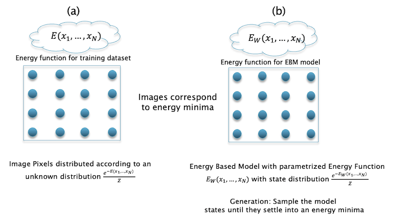
Figure 3: Image generation using EBMs
The above figure gives a high level overview of how EBMs can be used to generate images. Note that the nodes in the EBM correspond to pixels in the image. Given training data consisting of a bunch of images, we will assume that the pixels in an image follow a Boltzmann distribution $p(x_1,…,x_N)={e^{-E(x_1,…,x_N)}\over{Z}}$ for some unknown energy function $E(x_1,…,x_N)$.
The right hand side of the figure shows an EBM model with energy function $E_W(x_1,…,x_N)$, with corresponding Boltzmann distribution $p_W(x_1,…,x_N)={e^{-E(_Wx_1,…,x_N)}\over{Z_W}}$. We can consider that the nodes in the EBM model are interacting with each other, which results in the interaction energy $E_W(x_1,…,x_N)$, and ultimately the interactions settle down to an equilibrium in which the distribution of the pixels is given by the Boltzmann distribution. Thus the equilibrium state, which is that of lowest energy, also corresponds to states that result in images that look like those from the training dataset. During inference, sample images are generated by starting from a random state $(x_1,…,x_N)$ (which look like noise), and then using the sampling process to find the configuration that has the minimum energy. The model is considered to be trained if these sample images are similar to those in the training dataset. Sampling essentially results in finding a local minima of the energy function $E_W$, and its trajectory can be considered to similar to that of a particle moving in a force field with energy $E_W$.
Later in this article we will describe two ways by which the EBM model can be trained:
-
The maximum likelihood (MLE) algorithm chooses the parameters $W$ such that $p(x_1,…,x_N)\approx p_W(x_1,…,x_N)$ and this is basically the algorithm that Hinton used to train the Boltzmann machine. The modern more powerful version of the MLE algorithm that will be described in this article is called Diffusion Recovery Likelihood or DRL algorithm.
-
The score function for an EBM is defined as the set of derivatives ${\partial E\over{\partial x_i}}$ of the energy function with respect to the state. It is possible to sample from an EBM using knowledge of the score function alone, without knowing its energy function. Hence another way to train the EBM is by matching the score functions of the training dataset and the EBM so that ${\partial E\over{\partial x_i}}\approx{\partial E_W\over{\partial x_i}}$, and this results in an algorithm called Noise Conditioned Score Networks or NCSN.
Text to Image Generation
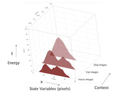
Figure 4: Variation of energy functions depending on the textual context
The process of image generation using an EBM is like a ball rolling downhill in a hilly landscape under the influence of the energy field $E_W$, but how does it find the ‘right’ valley to settle into? In other words, how can we specify what image to generate? This is the province of text to image models which turn a textual description into the corresponding image. Image to image models or text to text models (also called LLMs) also fall into this class, hence it constitutes a very important class of AI models.
The image generation process in these models can be understood as sampling that minimizes the energy function $E_{W}(x_1,…,x_N, c)$ where the variable $c$ is the latent vector representing the textual description. During inference, sample images are generated by starting from a text description $c$ and a random state $(x_1,…,x_N)$, and then using the sampling process to find the configuration that has the minimum energy for the given value of $c$. Each value of the text $c$ can led to multiple possible generated images, depending upon our choice of the initial random state configuration. Using the probabilistic point of view, this can be understood as matching the conditional probability $p(x_1,…,x_N\vert c)$ of the training data with the conditional probability $p_W(x_1,…,x_N\vert c)$ computed by the EBM model.
For a given context $c$, the energy $E_W(x_1,…,x_N,c)$ forms a function with multiple minima, such that each minima corresponds to images similar to those in the training set, just as before (see above figure). However the presence of the context means that all these images are constrained by it. For example if the context is “Images of dogs jumping over a fence” then the energy landscape with be limited to state configurations that correspond to this text.
Generative EBMs as Models for Biological Brains
This section consists of some speculation on my part on the subject whether the recent progress in EBMs can shed any light on the processing that goes on in our brains. Both our brains and the latest generation of ANNs seem to be doing similar things, but efforts to find ANN type mechanisms in the brain have not yielded much success so far. The brain itself has billions of neurons with trillions of connections between them, which is collectively referred to as the connectome. There are efforts underway to map the connectome to see whether it can offer some insight, but given the enormity of the task, the progress has been very slow. There has been one significant success though: Around 1960 the neuroscientists Hubel and Wiesel were able to map the circuitry that led from a cat’s eye to its neural cortex, and twenty years later this work served as the inspiration for the design of convolutional neural networks or CNNs. However no such neural structures have been found that are similar to the transformer architecture, and nor is there any evidence that the brain uses a backprop like algorithm for training its neurons.
In my opinion looking for signs of transformers or backprop in the brain is probably not the right way to approach the problem. It is more likely that the brain operates using EBM principles since these are firmly grounded on the physics of how a large number of nodes can interact with one another and create emergent behaviors. The interconnect topology between neurons is extremely complex and it is quite likely that its explanation will lie outside human comprehension for the forseeable future. However EBM theory tells us that what is important is not the interconnect topology, but the resulting energy function that results from the interactions. Indeed the properties of the energy function determine the information stored in the EBM and how it can retrieved. So perhaps this provides a clue that instead of trying to exactly map the connectome, we should be studying the brain at the level of its energy function instead. Even more interesting is the speculation that transformers don’t serve as a model for the connectome, but instead are really models for the energy function that emerges from the connectome.
But what about training, since there is no evidence of backprop in the brain? It is quite likely that training happens using a sampling type of algorithm of the type that EBMs use. These algorithms can be connected back to the synaptic learning rule that McCulloch and Pitts proposed back in the 1940s. If this indeed were to be the case, this would also explain why our brains are much more energy efficient than the current generation of ANNs, since thermodynamic based sampling can exploit the physics of the substrate, and thus can be faster as well as energy efficient.
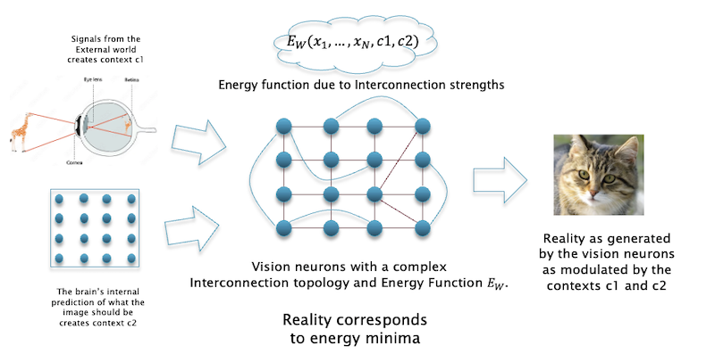
Figure 5: A Model for Biological Brains
With these ideas in mind, the above figure shows a proposed architecture for part of the brain that results in visual images. The image that see in front of us does not really exist in reality, in fact it is internally generated by our mind (for more on this topic read my article What would Kant think of LLMs). I am going to assume that there is a set of neurons in our brain whose state $(x_1,…,x_N)$ corresponds to an image that we see, lets call them the vision neurons. The process by which the vision neuron state actually gets converted into an image that we see is a deep mystery into which there is no insight at the present time, also called the hard problem of consciousness. I am proposing that the vision neurons have a dense interconnection architecture of the spin glass type, and furthermore the multiple minima of its resulting energy function $E(x_1,…,x_N)$ correspond to states of reality in the external world.
But how does the brain correlate the external reality with the state of the vision neurons, in other words how does it make sure that the image that it generates bears some correspondence to what is actually happening in front of us? A possible mechanism by which this is done is as follows, this is inspired by the text to image models discussed in the previous section: The light impinging on our retina leads to neuronal signals that are processed using the CNN like structure that Hubel and Wiesel discovered. This results in the signal getting converted into a configuration of neurons, lets call it the context $c1$. There is another set of neurons that make a prediction of what the image should be, lets call it the context $c2$. These context neurons then interact with the vision neurons to create the energy function $E_W(x_1,…,x_N,c1,c2)$, and the resulting minima of this energy function results in a configuration of vision neurons that result in what we see. Hence in some sense most of the information in the image that we see is already stored in the vision neurons of our brain, the sparse signals coming from our eyes merely serve as a pointer to choose the correct image. An excellent discription of how our external reality is internally generated can be found in Chapter 5 of Anil Seth’s book Being You. The EBM model that I just described serves as a mechanism by which the a dense inter-connection of neurons can do the generation. This mechanism also serves as a way in which we can conjure up images even with our eyes closed. There are portions of our brain that store memories, most likely in the hippocampus. The neural configurations of these memories can also serve as the context vector $c$ that triggers the vision neurons to create images for us.
We will talk about predictions using EBMs in detail in Part 4 of this article series, this will take us into the realm of world models and optimal control. This framework also incorporates how we take actions in the external world. If we want to take an action, lets say move our hand, the brain incorporates the effect of that action in the prediction $c2$, and then our muscles move to minimize the erroe between $c2$ and the state of the external world. For more information on this topic see Karl Friston’s work on the Free Energy Principle.
Just like for images, there is perhaps a corresponding part of the brain that is responsible for generating language, lets call it the language neurons. This comes with its own interconnection topology and energy function $E(x_1,…,x_N)$. The minima of this energy function correspond to words and sentences that correspond to thoughts that we are trying to verbalize. In analogy to images, words are like pixels, and a thought is a collections of words just as an image is a collection of pixels. But how do the language neurons decide on what thought to verbalize? This leads to the idea of a context $c$ which controls the language output by controlling the minima that the language energy function settles into. In this case the context can be one of several things:
- The context can be something that was uttered a moment ago, which results in a continuation of the thought. This also creates a way in which thoughts can be strung together in a sequence, thus opening the way to reasoning and world models. This topic is explored more fully in Part 4.
- The context can be an image, so for example image to language conversion.
These speculations lead to the idea that we can create a model of the brain by creating a dense interconnect network whose energy function corresponds to an ANN, such as the transformer. But what does this interconnect pattern look like? This seems to be an open question at present, but it is not an insurmountable one, and I expect to see progress in this area in the coming years. Clearly the interactions are more complex than the two node interactions in a spin-glass type model, and involve multiple nodes interacting with one another, and thus closer to the P-Spin or PSM type models described in Part 1. Are these more complex interactions biologically plausible? Interactions between biological neurons seem to be of the two node type, however one way to reduce higher node interactions to two node interactions is by introducing hidden nodes into the model, as done in the Boltzmann machine.
After all this speculation, lets get down to the nuts and bolts of how modern EBMs work, and we will start with Langevin sampling followed by training algorithms.
MCMC Sampling Using Langevin Dynamics
Early EBMs from the 1980s, such as the Boltzmann Machine, feature relatively simple energy functions
\[E_W = -\sum_i\sum_{j\lt i} w_{ij} \sigma_i\sigma_j - \sum_i b_i \sigma_i\]where $\sigma_i$ is the spin at node $i$, which can take values ${+1,-1}$, $w_{ij}$ is the symmetric strength of the interaction between nodes $i$ and $j$ and $b_i$ the threshold for activating node $i$. The spins in these networks are updated using Gibbs sampling
\[p(\sigma_k = 1\vert \sigma_1,..,\sigma_{k-1},\sigma_{k+1},...,\sigma_N) = p_k = {1\over{1 + e^{-\beta h_k}}}\]where $h_k = \sum w_{ki}\sigma_i + b_k$. Repeated sampling results in the network state gradually moving to an equilibrium configuration which corresponds to a local minima for the energy function. Gibbs sampling only works if we are able to compute this conditional probability, if the energy function is modeled by an ANN (such as those in the lower part of Figure 2) then clearly this procedure no longer holds.
Fortunately there is a way to sample from an EBM without knowing the inter-connection strengths between its nodes, and this is given by the iteration of the Langevin dynamics. The discrete time version of Langevin dynamics is given by the iteration
\[x^i_{n+1} = x^i_n -\eta {\partial \log p_W(x^1,_n,...,x^N_n)\over{\partial x^i_n}} +\sqrt{2\eta}\epsilon_n,\ \ n = 0,1,2,...\]Using vector notation this can also be written as
\[X_{n+1} = X_n -\eta \nabla_x \log p_W(X) +\sqrt{2\eta}\epsilon_n,\ \ n = 0,1,2,...\]where $X_n = (x^1_n,…,x^N_n)$ is the state vector and $\nabla = ({\partial\over{\partial x^1_n}},…,{\partial\over{\partial x^N_n}})$ is the differential operator. $X_0$ is usually initialized from the Gaussian distribution, $\eta>0$ is the step size and the noise vector $\epsilon_n$ is distributed according to the Gaussian $N(0,I)$. It can be shown that in equilibrium, the distribution of $X_n$ converges to $p_W(X)$ exponentially fast as $n\rightarrow\infty$ (see Roberts and Tweedie for a proof). Since in EBMs we want the distribution $p_W(X)$ to converge to the Boltzmann distribution, substituting $p_W(X) = {e^{-E_W(X)}\over Z_W}$ results in
\[X_{n+1} = X_n -\eta \nabla_x E_W(X) +\sqrt{2\eta}\epsilon_n,\ \ n = 0,1,2,...\]Note that by taking the derivative $\nabla_x p_W(X)$, the dependence on $Z_W$ goes away in the Langevin equation! The first two terms on the RHS of this equation are just the Newton method for finding the vector $X$ at which the function $E_W(X)$ is minimized (or equivalently the probability $p_W(X)$ is maximized), while the third term adds some noise to the process. Hence the overall effect is that of moving the system state to regions of lower energy (and higher probability), while the noise term enables the iteration to occassionally jump out of local minima so that there is a greater probability that the iteration ends near a deeper minima. This equation is also sometimes referred to as the Langevin diffusion, especially for its continuous time version.
The beauty of the Langevin diffusion is that enables us to generate samples from the distribution $p_W(X)$ without having to explicitly compute the partition function $Z_W$ or even the energy function $E_W$, all that we need are estimates of the score function $\nabla_x E_W(X)$. This frees us from the necessity of relating the energy function back to the inter-node interactions and enables sampling from arbitrarily complex energy functions. Note that unlike the Gibbs equation the Langevin equation can also be used for the case when the state $X_n$ is a collection of real numbers. Although not very well known yet, the Langevin diffusion is probably the most important equation in the modern theory of generative models.
Training EBMs Using Score Functions
Given a training dataset consisting of a collection of images, we will start with the problem of training an EBM model that generates new images that look similar to those in the training set. We will assume that the distribution of image pixels in the training dataset is given by the Boltzmann distribution with an unknown energy function $E$
\[p(x_1,x_2,...,x_N) = {e^{-E(x_1,...,x_N)}\over{Z}}\]Our EBM model in turn, has an equilibrium distribution given by its own energy function $E_W$ parametrized by weights $W$, given by
\[p_W(x_1,x_2,...,x_N) = {e^{-E_W(x_1,...,x_N)}\over{Z_W}}\]In order to make the generated images similar to those in the training set, we want to choose the model parameters $W$ so that $p(x_1,x_2,…,x_N)\approx p_W(x_1,x_2,…,x_N)$. This was the approach taken by Hinton and Sejnowski in their training algorithm for the Boltzmann machines, and they showed that the problem reduces to finding the maximum likelihood estimates of $W$. We will pursue this approach in the next section, but we will start with a simpler algorithm that is based on estimating the score function $\nabla_x E_W(x)$. This results in the problem of choosing $W$ to minimize the score matching error, also called the Fischer divergence, given by
\[L_{SM}(W) = {1\over 2}\sum_{i=1}^N E_{p(X)} ({\partial\log\ p_W\over{\partial x_i}} - {\partial\log\ p\over{\partial x_i}})^2 = {1\over 2} E_{p(X)}\vert\vert\ s_W(X) - \nabla_x \log\ p(X)\vert\vert_2^2\]where the score given by $s_W(X) = \nabla_x p_W(X)$. Note that we are using an ANN with parameters $W$ to model the score function directly, thus bypassing the need to model the energy function. This approach can be made to work, as first pointed out by Hyvarinen, but however runs into the problem of computing second order derivatives or the trace of Jacobian during the training process.
The big advance was made by Vincent in 2011 which he called denoised score matching or DSM and the critical idea was that of introducing noise into the training process. Vincent noted that the problem with minimizing $L_{SM}(W)$ is due to the intractability of $\nabla_x\log p(X)$. He proposed injecting noise into the data samples $X$ via a known conditional distribution $p_\sigma(X’\vert X)$ with scale $\sigma$. We then choose the model parameters $W$ so as to approximate the score of the noisy samples, by minimizing the loss function
\[L_{SM}(W,\sigma) = {1\over 2} E_{p(X')}\vert\vert\ s_W(X';\sigma) - \nabla_{X'} \log\ p_{\sigma}(X')\vert\vert_2^2\]where the distribution of the noisy sample is given by
\[p_{\sigma}(X') = \int p_{\sigma}(X'\vert X) p(X) dx\]Vincent showed that even though $\nabla_{X’} \log p_{\sigma}(X’)$ is intractable, it can be replaced by a tractable objective by conditioning on the distribution $p(X)$ of the original data samples, which results in the Denoising Score Matching (DSM) loss given by
\[L_{DSM}(W,\sigma) = {1\over 2} E_{p(X),p(X'\vert X)}\vert\vert s_W(X';\sigma) - \nabla_{X'} \log\ p_{\sigma}(X'\vert X)\vert\vert_2^2\]It can be shown that the value of $W$ that minimizes $L_{DSM}(W,\sigma)$ results in the the equation
\[s^*(X';\sigma) = \nabla_{X'} \log p_{\sigma}(X')\]and this is the same $W$ that minimizes $L_{SM}(W,\sigma)$.
When the noise level $\sigma$ is small,
\[s^*(X',\sigma)\approx \nabla_{X} \log p_{\sigma}(X)\]so that taking a small step along the noisy score direction $s^*(X’;\sigma)$ moves a noisy sample in roughly the same direction as a clean sample, which is the intuition behind why this technique works.
For the special case when $p_{\sigma}(X’\vert X)$ is Gaussian with variance $\sigma^2$ so that
\[X' = X + \sigma\epsilon\]and the noise vector $\epsilon$ is distributed according to $N(0,I)$, so that
\[p_{\sigma}(X'\vert X) = N(X'; X, \sigma^2 I)\]where $I$ is the identity matrix. It can be shown that the conditional score assumes the simple form
\[\nabla_{X'}\log p_{\sigma}(X'\vert X) = {X-X'\over{\sigma}}\]thus making the minimization of $L_{DSM}(W,\sigma)$ computationally feasible. The DSM loss simplifies to
\[L_{DSM}(W,\sigma) = {1\over 2} E_{p(X),p(X'\vert X)}\vert\vert s_W(X';\sigma) - {X-X'\over{\sigma}}\\vert\vert_2^2\] \[= {1\over 2} E_{p(X),\epsilon}\vert\vert s_W(X+\sigma\epsilon;\sigma) + {\epsilon\over{\sigma}}\\vert\vert_2^2\]Estimating $W$ by minimizing $L_{DSM}(W,\sigma)$ is a straightforward regression problem. The final step is to make the noise level $\sigma$ go to zero, so that
\[\nabla_{X'} \log p_W(X') \approx \nabla_{X} \log p(X)\]and the two score functions match.
Noise Conditional Score Networks (NCSN)
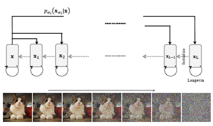
Figure 6: Illustration of a NCSN
The DSM algorithm has some shortcomings; in complex high dimensional energy spaces with lots of saddle points where the score function is close to zero, the Langevin iteration can stuck in sub-optimal regions. Even if it eventually manages to get out, it can take a long time to converge. The solution to this problem was proposed by Song and Ermon, and is basically a version of the simulated annealing algorithm that was described in Part 1. Recall that simulated annealing worked by starting the optimization at a high temperature so that the iteration had enough energy to jump out of shallow local minima and saddle points, and then gradually reducing the temperature to allow it explore deeper regions within larger valleys. Song and Ermon proposed a similar mechanism for DSM, which they called Noise Conditioned Score Networks (NCSN), where the noise was varied not through temperature, but by varying the variance $\sigma$ used in the DSM algorithm.
The NCSN algorithm is illustrated in the above figure. During training, noise is injected at multiple levels $\sigma_1,…,\sigma_L$, where $\sigma_1<\sigma_2<…\sigma_L$, and the idea is to train a score model $s_W(X,\sigma)$ that works for all $\sigma\in {\sigma_1,…,\sigma_L}$. The NCSN objective is given by
\[L_{NCSN}(W) = \sum_{i=1}^L \lambda(\sigma_i) L_{DSM}(W,\sigma_i)\]where
\[L_{DSM}(W,\sigma) = {1\over{2}}E_{P(X),P(X'\vert X)}[\vert\vert s_W(X',\sigma) - {X-X'\over{\sigma^2}}\vert\vert^2_2\]where $\lambda(\sigma_i)$ is a weighing function for each noise level. Minimization leads to a score model $s^{*}(X,\sigma)$ that can be used at at each noise level to recover the true score $\nabla_X\log p_{\sigma}(X)$ for all $\sigma\in {\sigma_1,…,\sigma_L}$.
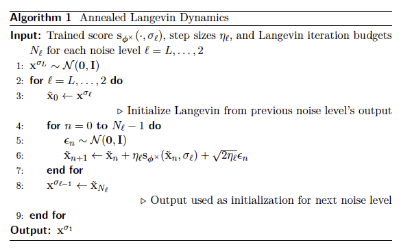
During the inference process, we start with a pure random sample $X_0$ distributed according to $N(0,I)$, and then the Langevin iteration is applied successively at each noise level $\sigma_l$ (starting from the largest $\sigma_L$) to sample from the distribution $p_{W}(X’;\sigma_l), l=L,L-1,…,1$. At each level the algorithm is iterated $K$ times, and the output from level $\sigma_l$ is used to initialize the next lower level $\sigma_{l-1}$. The iteration at the $l^{th}$ level is given by
\[X_{n+1} = X_n - \eta_l s_W(X_n,\sigma_l) + \sqrt{2\eta_l}\epsilon_n\]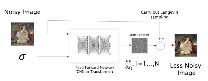
Figure 7: A single step of the denoising process using Langevin sampling using the score estimate
A single step of the de-noising process is illustrated above. The complete inference algorithm is given below (from Song and Ermon)
Training Using Maximum Likelihood Algorithm
The score based technique described in the previous section was able to generate images which are currently the state of the art in the field. However it does come with issue that it uses regression to estimate the score function, and this requires the use of the backprop algorithm. This contrasts with the earlier Boltzmann machine based image generation models whose operation was entirely based on the sampling operation. It would be nice if there was a way to equal the performance of the score based technique, while basing it entirely on Langevin or Gibbs sampling type operations, and without the use of backprop. It also brings us one step closer to a more energy efficient generative model, if the sampling operation can be implemented in an energy efficient manner.
The Maximum Likelihood (MLE) Algorithm
As before let $p(X)$ and $p_W(X)$ be the probability distributions for the training examples and the model respectively. Since it is an EBM, we can write $p_W(X)$ as
\[p_W(X) = {e^{-E_W(X)}\over Z_W}\]where $X$ is a vector $X=(x^1,…,x^N)$ and the partition function is given by $Z_W = \int e^{-E_W(X)} dX$ as usual. Assuming we are given $M$ training samples $X_1,…,X_M$, in order to learn this model using MLE, we have to maximize the log-likelihood function given by
\[L(W) = {1\over M}\sum_{i=1}^M \log p_W(X_i) = E_{p(X)}[\log p_W(X)]\]This can be written as
\[L(W) = -{1\over M}\sum_{i=1}^M E_W(X_i) - \log Z_W\]The maximization can be done by using the gradient ascent algorithm, $w_i \leftarrow w_i + {\partial L(W)\over{\partial w_i}}, i =1,…,P$, which can be written in vector form as
\[W\leftarrow W + \nabla_W L(W)\]but in order to do this we need to estimate $\nabla_W L(W)$ which can be done using the following steps.
Differentiation of $\log\ p_W(X)$ leads to
\[\nabla_W\log\ p_W(X) = -\nabla_W E_W(X) - \nabla_W \log Z_W\]The first gradient term $-\nabla_W E_W(X)$ can be evaluated by using an automatic differentiator. It can be shown that (see Song and Kingma for a derivation)
\[\nabla_W \log Z_W = E_{p_W(X)}[-\nabla_W E_W(X)]\]so that
\[\nabla_W\log p_W(X) = -\nabla_W E_W(X) + E_{p_W(X)}[\nabla_W E_W(X)]\]It follows that
\[\nabla_W L(W) = E_{p(X)}[\nabla\log p_W(X)] = -E_{p(X)}[\nabla_W E_W(X)] + E_{p_W(X)}[\nabla_W E_W(X)]\]The first term in the derivative is evaluated by using samples from the training dataset which are distributed according to $p(X)$, while the second term is evaluated by using samples generated by the model, which are distributed according to $p_W(X)$. The first term decreases the energy for data points that belong to the training set, while the second term increases the energy for data samples that are generated from the model. For the case when $E_W(X)$ is a expressed by an ANN such a transformer or a CNN, this derivative can be computed using automatic differentiators.
The MLE based technique hinges on getting samples from the model which are distributed according to $p_W(X)$ and since we can no longer use Gibbs sampling, we resort to using Langevin sampling instead
\[X_{n+1} = X_n - \eta\nabla_X E_W(X_n) +\sqrt{2\eta}\epsilon _n\]where $\epsilon_n$ is drawn from a normal distribution $N(0,I)$. The gradient $\nabla_X E_W(X)$ can be computed using automatic differentiators.
This algorithm suffers from the same issues that plagued the Boltzmann machine and led to long sampling times thus limiting its scalability to few hundred nodes at most. Gap, Song et.al. proposed a way to get around this problem, and this is covered in the next section.
Recall that in Part 2 we showed that for the Boltzmann machine the gradient for the loss function is given by the Hebbian learning rule
\[{\partial L(W)\over{\partial w_{ij}}} = \beta (<\sigma_i\sigma_j>_{data} - <\sigma_i\sigma_j>_{model})\]This is a special case for the more general equation above, and can be recovered by noting that the energy function for the Boltzmann machine is given by
\[E = -\sum_{i}\sum_{j\lt i}w_{ij}\sigma_i\sigma_j - \sum_{i}\sigma_{i} b_i\]The Diffusion Recovery Likelihood (DRL) Algorithm
Just as for the NCSN algorithm used with score matching, the DRL algorithm is also based on the idea of injecting noise at various levels of intensity during the sampling process. Before we describe this, lets look at MLE for the case when the data samples $X$ are perturbed by Gaussian noise so that
\[X' = X + \sigma\epsilon\]where as before $\epsilon$ is distributed according to $N(0,I)$. We will try recover the data samples $X$ from the noise samples $X’$ by using an EBM model with parameters $W$. If as before, $p_W(X)$ is distributed according to
\[p_W(X) = {e^{-E_W(X)}\over Z_W}\]then using Bayes rule it can be shown that the conditional probability $p_W(X\vert X’)$ is distributed according to
\[p_W(X\vert X') = {1\over Z'_W} e^{-E_W(X) - {1\over{2\sigma^2}}\vert\vert X'-X\vert\vert^2}\]where $Z_W = \int e^{-E_W(X) - {1\over{2\sigma^2}}\vert\vert X’-X\vert\vert^2} dX$ is the partition function for the conditional EBM. The extra quadratic term causes the resulting energy landscape to be localized around $X’$, thus making it less multi-modal and easier to sample from. When $\sigma$ is small, the conditional distribution is approximately single mode Gaussian.
We can define a maximum likelihood function $J(W)$ for the conditional distribution, given by
\[J(W) = {1\over M}\sum_{i=1}^M \log p_W(X_i\vert X'_i)\]and the objective is to recover the clean sample $X_i$ from the noisy sample $X’_i$ by maximizing this likelihood. It can be shown that the corresponding Langevin sampling is given by
\[X_{n+1} = X_n - {\eta}[[\nabla_X E_W(X_n) - {1\over{\sigma^2}}(X'_n-X_n)] +\sqrt{2\eta}\epsilon _n\]When this iteration converges the resulting $X$ value will be distributed according to $p_W(X\vert X’)$.
The model is then updated according to $W\leftarrow W + \nabla_W L(W)$, where the gradient is given by
\[\nabla_W L(W) = -E_{p(X\vert X')}[\nabla_W E_W(X)] + E_{p_W(X\vert X')}[\nabla_W E_W(X)]\]Note that the term ${1\over{\sigma^2}}(X’_n-X_n)$ does not appear in this equation since its derivative with respect to $W$ is zero. It can be shown that given enough data, maximizing $J(W)$ leads to unbiased estimates of the parameters $W$ (see Appendix A2 in Gao, Song et.al. for a proof).
Since the recovery likelihood method described to recover $X$ from $X’$ works well only well the noise level $\sigma$ is small, we can use the same trick as in the NCSN algorithm, and learn a sequence of recovery likelihoods, each of which has a small noise level. In order to do this, a data sample $X(0)$ is perturbed in a sequence of steps to create noisy samples $X(1),…,X(T)$ given by
\[X(t+1) = \sqrt{1-\sigma^2(t+1)} X(t) + \sigma(t+1)\epsilon_{t+1},\ \ t=0,1,...,T-1\]Defining $Y(t) = \sqrt{1-\sigma^2(t+1)} X(t)$, we get a sequence of conditional EBMs
\[p(Y(t)\vert X(t+1)) = {1\over{Z'_W(X(t+1),t)}} e^{-E_W(Y(t),t) -{1\over{2\sigma^2(t)}} \vert\vert X(t+1)-Y(t)\vert\vert^2}\ \ \ \ t=0,1,...T-1\]where $E_W(Y(t),t)$ is defined by an ANN with parameters $W$ which is conditioned on $t$. The corresponding Langevin sampling of the conditional distribution is given by
\[Y_{n+1}(t) = Y_n(t) - \eta[\nabla_Y E_W(Y_n(t),t) - {1\over{\sigma^2(t)}} (X(t+1)-Y_n(t))] +\sqrt{2\eta}\epsilon _n,\ \ \ \ \ \ \ \ \ \ \ \ \ \ \ \ (17)\]Once we have a sample from the conditional distribution $p_W(Y\vert X(t+1))$, it is plugged into the expression for the gradient of the log likelihhod loss function
\[\nabla_W L(W,t) = -E_{p(Y\vert X(t+1))}[\nabla_W E_W(Y,t)] + E_{p_W(Y\vert X(t+1))}[\nabla_W E_W(Y,t)]\]which then gets plugged into $W\leftarrow W + \eta \nabla_W L(W,t)$ to estimate the model weights. Given $X(t+1)$, the $Y$ sample is drawn from the training data for the first expectation, while it is drawn from the conditional distribution $p_W(Y\vert X(t+1))$ defined by the model with parameters $W$ using the Langevin sampling equation given above, for the second expectation.
Note that the DRL training algorithm does not involve the use of the backprop algorithm, and the learning happened by way of sampling. This makes it somewhat of a rarity in the modern world of AI systems, and also increases the possibility that the brain employs something similar (especially since no evidence of backprop has been found in the brain).
The complete training and inference algorithms are given below. Note that during inference we start with a pure noise image $X(T)$, and the gradually denoise it by successively sampling from the conditional probability $p_W(X(t)\vert X(t+1))$ until we get to $X(0)$. The output $X(t)$ of step $t$ is then fed into the fed into the next step to estimate $X(t-1)$.
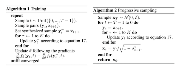
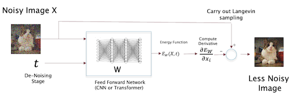
Figure 8: Illustrating a single stage of the DRL algorithm
The above figure summarizes a single stage of the DRL algorithm. Note that in this case we are explicitly computing the energy function and then differentiating it to do the Langevin sampling.
Conditional Generation Models
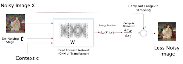
Figure 9: Context dependent DRL algorithm, with context $c$
The image generation process can be conditioned on other latent variables, and this results in a very important class of EBMs. For example text to image models fall into this class, and indeed all important applications of generative models involve some type of conditional generation. Even LLMs can be considered to be a type of conditional EBM model, in which the next chunk of generated text is conditional to the previously generated chunk. In Part 4 of this series of articles we will come across world models used in reinforcement learning, which involve prediction of the next system state, and this can be considered to be a generative problem conditioned on the current state and the action taken by the agent.
With context dependence the objective is to maximize the log likelihood of the conditional distribution
\[L(W) = {1\over M}\sum_{i=1}^M \log p_W(X_i\vert c) = E_{p(X)}[\log p_W(X\vert c)]\]where $c$ is the context vector. Assuming $p_W(X\vert c)$ is given by a Boltzmann EBM with energy function $E_W(X,c)$, the expression of the gradient for this function becomes
\[\nabla_W L(W) = -E_{p(X\vert c)}[\nabla_W E_W(X,c)] + E_{p_W(X\vert c)}[\nabla_W E_W(X,c)]\]The above figure a single stage $t$ of the DLR de-noising process. Note that the main difference from the un-conditional case is the presence of an additional input $c$, so that the energy function that the model computes is now $E_W(X,t,c)$. The best way for introducing this conditioning has been found to be by using transformer based energy models. In this case the conditioning is done by using the operation of cross attention in the transformer stack, with key and value (KV) pair coming from $the context $c$, and the query (Q) coming from the lower layer of the transformer stack.
After the training is complete, new images are generated by fixing the context $c$ and starting from a random image $X(T)$, and then gradually denoising it using Langevin sampling. Note that more than one possible image can be generated for a given $c$, and this is a function of the initial starting point $X(T)$.
Figure 10:
An example of conditional text to image generation using DRL type system is shown in the above figure. We can see that the context is being input in each stage of the de-noising pipeline.
The DRL algorithm can be applied to the Boltzmann machine as well, this is discussed in the next section.
Hardware Implementation of EBMs
We have shown that EBMs can be used to implement state of the art generative models, and this leads to the question of whether there is any particular benefit in using them (vs non-EBM generative models). Sara Hooker, an engineer at Google, published an interesting essay The Hardware Lottery a few years ago in which she pointed out the most dominant architecture at any point in time is a result of synergy between available hardware and the software that gets written to use it. This is particularly true for AI systems as recent history shows. Until about 2010 deep learning was one of the many approaches to AI, and it was not clear which approach would win out. In 2012, Hinton’s team showed that Graphical Processing Units or GPUs are very well suited for the backprop algorithm, and as a result it became possible to scale up the size of systems that could be trained using backprop by orders of magnitude, thus resulting in the current AI wave. Unfortunately GPUs do not result in the same compute acceleration when used for EBMs, since the basic operation in EBMs is sampling which cannot be parallelized using GPUs. State updates using sampling is an inherently serial node by node operation even when implemented on GPUs.
Then the question arises if we can design an equivalent of a GPU for EBMs, i.e., an hardware architecture that is specialized to accelerate sampling. Also, is there any benefit of pursuing this line of work vs just sticking to GPU based systems? The holy grail is a potential decrease in energy consumption. GPU based systems are very energy intensive, and it is often pointed out that biological EBM systems, such the brain, are able to do equivalent work with much lower power consumption. If the new EBM hardware implementations are able to approach state of the art performance with much lower energy consumption, then this will constitute a genuine advancement.
We will look at a few approaches for doing this that are based on analog computing technology. This field is in its infancy, and current systems still have a long way to go before they can realize their full potential.
Scaling Up Boltzmann Machines: The Extropic System
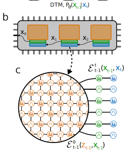
Figure 11: The Extropic Implementation for Boltzmann Machines
Extropic is a well funded start-up, founded by ex-members of Google Brain. Their initial design, which they announced in October 2025, had several new ideas for scaling up Boltzmann machines. They point out in their research report that there are two main challenges with scaling up Boltzmann machines:
1) Algorithmic problem: The usual way of training Boltzmann machines using the equation
\[{\partial L(W)\over{\partial w_{ij}}} = \beta (<\sigma_i\sigma_j>_{data} - <\sigma_i\sigma_j>_{model})\]runs into the problem of excessively long mixing times, where the Gibbs sampling procedure takes a long time to converge. This is an algorithmic issue and would persist even if the sampling were to be made more efficient using hardware. Fortunately this problem can be addressed using the DRL algorithm as we pointed in the previous section. This works by using a multistage architecture, where each stage tries to recover a de-noised version of the prior stage. The gradient of the MLE function $L(W)$ is computed using
\[{\partial L(W)\over{\partial w_{ij}}} = \beta (<\sigma_i\sigma_j>_{p(\sigma\vert\sigma(t+1))} - <\sigma_i\sigma_j>_{p_W(\sigma\vert\sigma(t+1))})\]The $\sigma$ value in the first expectation is sampled from the training dataset, while it is sampled from the conditional distribution $p_W(\sigma\vert\sigma(t+1))$ in the second expectation. This results in a multi-stage sampling operation (see above figure), where at each stage the system samples from a conditional probability distribution that is much easier to sample from. The top part of the figure shows their proposed hardware implementation, with multiple Boltzmann machines chained together in a serial fashion (for the backward flow of the DRL algorithm). Hence each of the hardware units is used to sample from a conditional Boltzmann distribution, where the conditioning is based on the output of the sampling in the prior stage. The states in the Boltzmann machine are color coded, with the orange corresponding to the hidden nodes, green corresponding to output nodes for the stage and blue corresponding the output nodes from the prior state. The bottom part of the figure shows details of a Boltzmann machine in one of the stages, once again showing the three kinds of nodes.
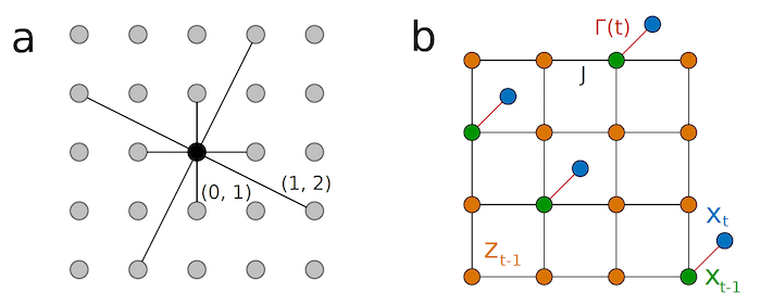
Figure 12: Inter-node Connections
The above figure goes into more detail about how the node interconnections are done. The system allows for both nearest neighbor as well as long range connections that can specified by the user, an example of which is shown on the left hand side. In order to do the denoising, the output from the prior stage, shown in blue, is fed into the output nodes for the current stage, shown in green, and these nodes are also interconnected with the hidden nodes shown in orange. The goal of the Extropic architecture is to have an arbitrary inter-connection pattern and still be able to sample efficiently. The current implementation is not quite there yet, since they simulated the system in software using a restricted Boltzmann machine type architecture (which allows for efficient Gibbs sampling in software).
The system is trained by by introducing noise at multiple levels, and then trying to recover the de-noised system from the noisy state. If the state is continuous, noise is introduced a Gaussian distribution as we have seen, but now we will have to use a discrete noise equivalent. Extropic does this by modeling the noise generation using a Markov chain, please Appendix A of their paper for details. They showed that samples of the noisy system can be generated by using a Boltzmann machine whose equilibrium distribution is the same as that of the Markov chain.
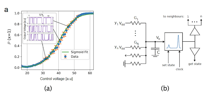
Figure 13: Random Number Generator and Node Implementation
Extropic’s implementation of the Boltzmann machine is based on a Random Number Generator (RNG) in CMOS. This was built by leveraging the shot-noise dynamics of sub-threshold transistors, and resulted in a sigmoidal response to a control voltage as shown in part (a) of the above figure. The output voltage, examples of which are shown in the inset diagram in part (a), is periodically sampled to generate a random stream of 1’s and 0’s.
Extropic is in the process of integrating its RNG with other components to create a single node of the Boltzmann machine, a schematic of which is shown in part (b) of the figure. Each node has a set of inputs from the neighboring nodes which is combined to produce a control signal that is used to bias the RNG circuit. The RNG is then sampled to produce a 0 or 1, that is in turn fed into the neighboring nodes. Extropic estimates that they can fit 1000X1000 grid of these nodes within a 6mm x 6mm chip.
Other Boltzmann Machine Implementations: P-Bit Based Systems (UCSB, Purdue)
The p-bit based approach to Boltzmann machine is the outcome of (ongoing work) at Purdue and UCSB, and good overview can be found in this paper. The overall objective of this project is the same as that for the Extropic system, the main difference being the technology that the p-bit group is pursuing to implement the system in hardware. As opposed to CMOS, the p-bit implementation uses Magnetic Tunnel Junction (MTJ) technology which is also used for in MRAMs (which are a new kind of dense nonvolatile memory being deployed at major semiconductor fabs). Hence it may be possible to build dense arrays of p-bits using the same process used for building MRAMs, this work is still ongoing. Using this technology it may be possible to build a Boltzmann machine in which all the nodes can update their state completely asynchronously, thus avoiding the use of RBMs.
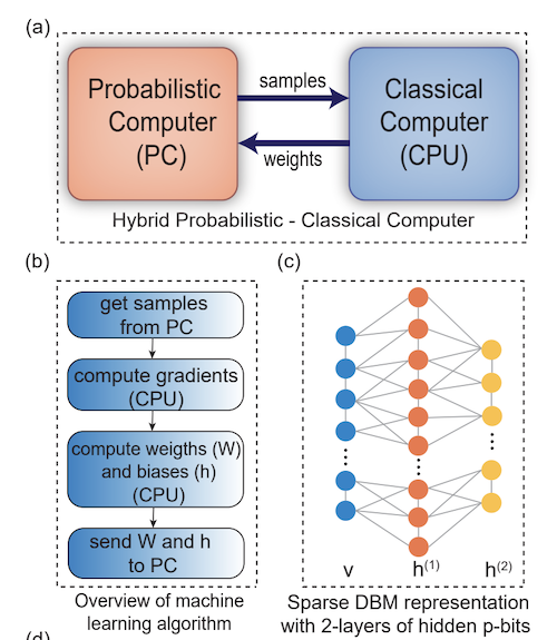
Figure 14: A hybrid computer scheme with probabilistic and classical computers
A hybrid computer featuring both probabilistic (Boltzmann machine) and classical parts is shown in the above figure. The Boltzmann machine is used to do fast and efficient sampling, while other parts of the training algorithm, such as the contrastive divergence calculations are carried out by the classical computer.
Since both Extropic and p-bit systems are mainly focused on building Boltzmann machines with binary 1 or 0 nodes values, what about systems of the type that we spent most of this article discussing? These involve continuous states, and require the use of Langevin sampling. Normal Computing is another startup that is building devices that can simulate the Langevin equation. More details about their system can be found here.