Encounters with Extreme Randomness: The Story of Brownian Motion
Contents
- Introduction
Two New Sciences - From Brownian Motion to the Wiener Process
- Stochastic Calculus and the Ito Integral
- Ito’s Formula
- Modeling the Stock Market
Does the Stock Market Follow a Wiener Process - Image Generation Using the Langevin Diffusion Process
- Is there a Connection with Quantum Mechanics?
Introduction
Figure 1: Brownian Motion
In 1827 the Scottish botanist Robert Brown was peering through his microscope at minute particles of pollen suspended in a drop of water, when he noticed something strange. The pollen particles seemed to be moving about randomly, with no preferential direction. That being the age of Newtonian Mechanics, Brown looked for a force that might be causing the particles to move, but he couldn’t find any that was visible. This phenomenon was named after him, and in fact most of us have seen particles of dust dancing around in a beam of sunlight in a darkened room, which is another example of Brownian Motion.
The cause of the random motion remained a mystery until 1905, when the young Albert Einstein came up with a satisfactory explanation in his very first published paper. Einstein theorized that the pollen particles where being pushed around by the molecules of water, which are too tiny to be seen under a microscope. At any point in time, there are slight imbalances in the number of water molecules exerting pressure on the pollen grain from various directions, as a result of which it gets pushed around randomly as time goes on. The question arises, how far does a pollen particle travel in time duration $t$? Since it is constantly changing direction, Newton’s Law’s of Motion are of certainly no use here. In fact it could be seen, that the particle covered randomly distributed distances in the same time duration, which implies that its motion could only be analyzed using the tools of probability theory. Robert Clerk Maxwell and others had introduced probabilistic thinking into Physics a few decades earlier with their Kinetic Theory of Gases. This theory though tried to predict macro properties such as pressure, and not the movements of individual particles. In this case we are interested in the random motion of a single particle, and this was something new to Physics. Nevertheless Einstein was able to use the tools of Kinetic Theory to show that that motion of the particle follows a well known statistical law, that of the Normal or Gaussian distribution, and that the average distance the particle moves in time $t$ is proportional to $\sqrt{t}$.
Unbeknownst to Einstein, Brownian Motion had already been analyzed five years earlier by the French mathematician Louis Bachelier in the context of a model for the stock market. There is a deep connection between the random wriggling of the pollen particles that Brown saw, and the movement of securities in the stock market, they share the same mathematical model, called the Wiener Process. In our own Artificial Intelligence age, the operation of the most popular image generation tools such as Dall-E-2 from OpenAI is also based on the very same Wiener Process!
Two New Sciences
At the dawn of the 20th century, there were two new sciences that were launched. One of them of course, was Quantum Mechanics, that came into existence with Max Planck’s 1901 paper on Black Body Radiation. The other less well known one, was the science of random processes, and this was initiated in his PhD Thesis by Louis Bachelier, also around the same time. Quantum Mechanics of course went on the upend our ideas of Physics and reality in general, but what about Bachelier’s discovery? This article is on precisely this topic.
The science of random events, or probability theory, was founded in the 17th century by the French mathematician and philosopher Blaise Pascal who was the first one assign numbers to notions such as the probability of winning at a game of chance. For example if we were to toss a 6-headed dice then the probability that it will result in the number 4, is ${1\over 6}$, and these probabilistic outcomes are given the name random variables. This was further developed in the 18th century, with the name most associated with it being the Swiss mathematician Jacob Bernoulli. Bernoulli initiated the idea of a repeated random trial, which was the first step towards the definition of a random process. For example if we toss a coin N times, he gave a formula for the probability that $n$ of those are heads and the remaining $N-n$ are tails, now called the Binomial Distribution.
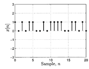
Figure 2: Discrete Time Random Processes: Outcome of a Sequence of Coin Tosses
But what if we were to look at an infinite sequence of coin tosses, this then becomes a (discrete valued) random process. An example of such a random process is shown above, it is created by tossing a coin multiple times, with heads represented by the random variable 1 and tails by 0.
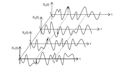
Figure 3: Continuous Time Random Processes
Extending this idea further, what if the random quantity evolves continuously in time? This then becomes a continuous time random process, also called a stochastic process, and an example of this is shown the above figure. You can think of these curves as being created by the Brownian Motion of a pollen particle whose movement is confined to just one dimension, either up or down along the y-axis, or the variation in the stock price for a company over time. Note that there are several curves shown in the figure, and each of them represents a possible time evolution of the random process when starting from the origin at $t=0$, these are called sample paths. They constitute the different outcomes in time for a random process and just as we assign a probability to an individual event, for example the probability of getting a heads when tossing a coin, we now assign a probability to the entire sample path as a whole. There are two ways to look at these curves:
- In terms of the time evolution of the random process, as captured in a single sample path, say $X(t)$, or
- By fixing the time $t$, and then looking at the values of the random process over the the collection of sample paths. This is shown by the two dotted lines in the figure for the case when time has been fixed at $t_1$ and $t_2$. In this case, we no longer have a random process, since the time evolution is lost, and instead we end up with the random variables $X(t_1)$ and $X(t_2)$.
The analysis of a continuous time random process is exponentially harder than the discrete time version since, unlike the case of tossing a dice that only has six possible outcomes, the set of possible outcomes is the space of continuous functions which is uncountably infinite. Consequently very little progress had been made in this area by 1900 and part of the reason was that there was no connection made between probability theory and the rapidly developing methods in analysis that had resulted in developments such as the Borel and Lebesgue Measures and the Lebesgue Integral towards the end of the 19th century which enabled mathematicians to handle spaces consisting of an infinite number of elements. The major contribution that the 20th century mathematicians made to the science of randomness, is precisely this connection and it laid the science of random processes on a firm foundation, by connecting it with the rest of mathematical analysis. This process started with Bachelier, and was completed two decades later with great Russian mathematician Andrei Kolmogorov’s axiomatization of probability theory which made it possible to talk about probability spaces that have an uncountably infinite number of elements. The space of functions that evolve randomly and continuously in time, which is precisely what a random process is, is a special case of these type of probability spaces. This has an interesting echo with Quantum Mechanics that also took about two decades two mature from Planck to Heisenberg and Schrodinger.
Kiyosi Ito was a Japanese mathematician who made the next important advance in the theory of random processes by founding the field of stochastic calculus. Working in wartime Tokyo during the 1940s, he came up with the idea of extending the idea of the integral to the case when the integration is done with respect to the random fluctuations of Brownian Motion, and this is now called the Ito Integral in his honor. I found this to be a totally mind blowing concept when I first learnt about in grad school in the late 1980s, and even today I consider it a privilege that I understand what it means. This idea was very influential since it allowed mathematicians to build more complex random processes by using Brownian Motion as a basic building block. This laid the foundation for several important applications of random processes that happened in the following decades.
But how important are these random processes in practice? Well, the most famous example of a randomly evolving continuous time process is the stock market, and this is precisely what Bachelier studied in his 1900 thesis. His work was essentially lost until the 1950s, when it came to the attention of the eminent economist Paul Samuelson, who built on Ito’s work and applied it to create a model for the stock market called the Geometric Brownian Motion. Later in the early 1970s the economists Fischer Black and Myron Scholes used Ito and Samuelson’s work to create a model for pricing stock options. This resulted in a partial differential equation named after them, whose solution is probably the most important mathematical result in use in Wall Street trading today. In fact I recently came across a list of the most important equations in science, and the Black-Scholes equation was listed along with others such as Maxwell Equations for electromagnetism and Schrodinger’s Equation for the quantum wave function.
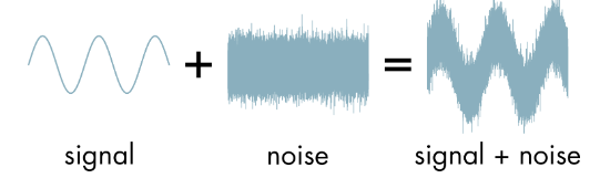
Figure 6: Signals in Noise
Brownian Motion has evolved into a powerful tool for modeling random phenomena. Whenever the need arises to capture the randomness that exists in fields such as communications system or electrical circuits, Brownian Motion is the go-to model that engineers use. An example of a deterministic signal subject to random noise is shown in the above figure. The clean signal is transmitted, while the noise is added during the course of transmission over a communications channel and the Filtering Problem looks at ways in which the signal can be extracted from the noise at the receiver. Norbert Wiener (more about him in the next section) and Richard Kalman are names associated with the solution to the filtering problem.
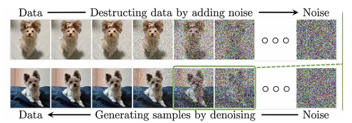
Figure 6: Training a Neural Network to generate images using random processes
But the most interesting, and surprising, application of Brownian Motion has happened within the last decade, when it was used to create a Neural Network model that can generate realistic images and videos. This model outperformed all competing methods, and it has become the most prevalent image and video generation model in use today. This topic is treated in greater detail later, but a rough idea of how it done can be seen in the above figure. The top row shows the process of adding incremental random noise to an image, until it becomes indistinguishable from pure noise. The bottom row trains the Neural Network by learning how to recover the original image from noise. Once the network is trained, it can generate new images by starting from a noise sample.
There was one name that I didn’t mention in my brief survey of mathematicians who have contributed to the theory of the Brownian Motion, and it is that of Norbert Wiener. This is quite a big omission since the terms Brownian Motion and Wiener Process are often used inter-changeably. Strictly speaking Brownian Motion is the physical phenomenon that Robert Brown discovered and Einstein analyzed, while the Wiener Process is a mathematical model for it and this is the terminology that I will use in the rest of this article. Norbert Wiener was the first one to do a rigorous mathematical analysis of Brownian Motion in the early 1920s, and abstracted it to create the mathematical notion of a Wiener Process. He proved several important properties for it, such as the fact that its sample paths are continuous in time, while at the same time its derivative does not exist anywhere. Wiener was a child prodigy who got his PhD from Harvard at age 19 and spent his career teaching at MIT. His work spanned mathematics, both pure and applied, as well philosophy and towards the latter part of his life what we call Artificial Intelligence (he called it Cybernetics). He contributed more than anyone else to the emerging field of Signal Processing, and was a big influence on the later work of Claude Shannon and John von Neumann.
So why is the Brownian Motion or the Wiener Process so useful in so many different applications? We will see later in this article, that it can be regarded as a prototypical continuous time random process. As soon as we constrain a random process to be continuous and have random increments that are independent, then only one process can result, namely the Wiener Process. In some sense the Wiener Process is the most random thing that one can think of, since it is continuously changing direction, no matter how small the interval we are examining. In fact there have been attempts made to link it to Quantum Mechanics, as a way in which the randomness in the latter can be explained by modeling a quantum particle like a version of a randomly moving pollen grain, we will cover this in the last section of this article.
The theory of a random process in continuous time was not sufficiently well developed when Wiener was working on the problem in the early 1920s, and had to wait for Kolmogorov’s axiomatization of Probability Theory ten years later. During the 1950s Monroe Donsker gave a highly intuitive explanation of how the Wiener Process arises as a limiting case of a simpler random processes, and this is what I am going to describe in the next section.
From Brownian Motion to the Wiener Process
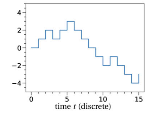
Figure: The Random Walk Process: Outcome of a Coin Tossing Experiment
Lets start with a very simple process, that of tossing a coin. Let the random variable $X_n$ be the result of the $n^{th}$ toss, and assign $X_n = 1$ if the result is a heads and $-1$ to tails. Define $S_n$ to be the random sum given by
\[S_n = X_1 + X_2 + ...+ X_n,\ \ \ n = 1,2,...\ \ \ and \ \ \ S_0 = 0\]If we interpolate in a step-wise fashion between successive values of $S_n$ by introducing time as a variable, then it results in the continuous valued random process shown in the above figure, which shows one possible sample path that can result. The random sum has the interesting property that once we know the value of $S_n$, the future evolution of the process is completely independent of what happened prior to the $n^{th}$ toss. These type of processes, in which the future is independent of the past given the present, form an important category called Markov Processes and the Wiener Process belongs to it.
The step-wise continuous random process can be defined using the function $W^n(t)$ as follows:
\[W^n(t) = S_{\lfloor t\rfloor}\ \ \ \ t\ge 0\]Note that the floor function $\lfloor t\rfloor$ results in the smallest integer less than or equal to $t$ and the resulting process is called s a Random Walk. It is created by defining the function $W(t), t\ge 0$ such that it is equal to the random sum $S_i$ at time $t=i$ and then maintains this value until it gets to the next point $i+1$, at which point it makes the next random jump equal to $X_{i+1}$.
So we have a continuous time process that seems to be evolving randomly, but it is not quite a Brownian Motion yet. How can we go about creating a more exact model? Brownian Motion exhibits much faster changes in direction compared to the Random Walk, and also successive changes happen much quicker in time. One way to accomplish these goals is by doing the following:
- Restrict the Random Walk to the time interval $t\in [0,1]$ so that the random jumps occur at at the $n$ time instants given by ${1\over n}, {2\over n},…,{n-1\over n}, 1$. Hence as $n$ increases the jumps happen faster and faster.
- Scale the random sums by ${1\over{\sqrt{n}}}$ so that as $n$ increases, the jumps in the $S_n$ values become smaller, i.e., the particle covers smaller and smaller distances with each change of direction.
This results in the scaled Random Walk given by
\[W^n(t) = {S_{\lfloor nt\rfloor}\over{\sqrt{n}}}\ \ \ 1\le n\le N,\ \ \ 0\le t\le 1\]Note that $W_n(t), 0\le t\le 1$ is equal to the scaled random sum ${S_i\over{\sqrt n}}$ at $t = {i\over n}$ and then maintains this value until it gets to $t = {i+1\over n}$, at which point it takes the next jump.
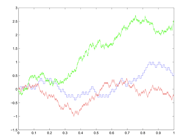
Figure: Scaled and Interpolated Random Sums over $0\le t\le 1$ for n = 100 (blue), n = 400 (red) and n = 10000 (green)
The figure above three different sample paths for $W^n(t)$ over the interval $[0,1]$, with the gap between successive changes in direction becoming smaller and smaller as $n$ increases. As $n\rightarrow\infty$, Donsker’s Theorem says that $W^n(t), 0\le t\le 1$ converges to a Wiener Process. What does it mean to take the limit $n\rightarrow\infty$? Since $W^n(t)$ is constrained to be in the interval $[0,1]$, it means that successive jumps are happening faster and faster, and in the limit they are happening over the continuum $t\in [0,1]$. Since each jump results in a change of direction for $W^n(t)$, it follows that in the limit, the change of direction is happening at each and every time instant! This is a bit difficult to visualize, but essentially this also means that in the limit a sample path of the Wiener Process $W(t), 0\le t\le 1$ does not have a derivative at any point in the interval $[0,1]$ (since the derivative is not defined at points at which the direction of a function changes).
There is a bit of ambiguity in the notation since $W(t)$ can refer both to the sample path of the random process over the interval $[0,1]$, as well the random variable $W(t)$ at time $t$. We will use the convention that $W(t)$ refers to the function defined over an interval such as $[0,1]$, while $W_t$ refers to the random variable at time $t$.
We now provide some heuristic arguments to show that the Random Sum Process $W^n(t)$ converges to the Wiener Process $W(t)$ as $n\rightarrow\infty$. But before we do that, the following question has to be answered: What does convergence mean when the objects we are talking about are random processes? Lets first consider what consider what convergence means in the context of random variables. Recall that we defined the random sum $S_n = X_1+X_2+…+X_n$ such that each $X_i$ was the outcome of a coin toss, but we can extent this to the more general case where the $X_i$ are arbitrary random variables with mean $m$ and variance $\sigma^2$. We will assume the $X_i$ are independent of one another, and furthermore thay are all identically distributed.
Under these conditions can we say anything about the convergence of the scaled version of this sum given by ${S_n\over\sqrt{n}}$? We certainly can, and this is one of the most famous results in probability theory called the Central Limit Theorem or CLT. It says that the probability distribution of ${S_n\over\sqrt{n}}$ converges to the Normal or Standard Gaussian Distribution $N(m,\sigma^2)$. More precisely
\[{S_n\over\sqrt{n}} \xrightarrow[\text {}]{\text{D}} {1\over\sqrt{2\pi\sigma^2}}e^{-{(x-m)^2\over {2\sigma^2}}}\ \ \ as\ \ \ n\rightarrow\infty\]This kind of convergence for random variables is called convergence in distribution or weak convergence and is denoted by $\xrightarrow[\text {}]{\text{D}}$ in the equation. It basically says that in the limit, we may not be able to tell the precise value to which ${S_n\over\sqrt{n}}$ will converge to (which is the traditional idea of convergence for a deterministic series), but we can give precise estimates of the probability that it falls within a specified interval, say $[a,b]$, and this is given by the Normal Distribution. In the rest of this section we will assume that $m = 0$ and $\sigma = 1$.
Can we define a similar type of weak convergence result for random functions $W^n(t), 0\le t\le 1$ as $n\rightarrow\infty$? This is a difficult problem to solve since now we are now talking about a probability space consisting of functions. A whole host of brilliant minds worked on this problem in 1950s, the most prominent names being Donsker in the US, Skorokhod, Kolmogorov and Prokhorov in the USSR. For those of you wanting to get deeper into this topic, there are several excellent books available, in particular “Convergence of Probability Measures” by Patrick Billingsley is standard reference for the theory of weak convergence over functional spaces.
In this article I will give some heuristic arguments for this convergence and I will start by showing a couple of important properties for $W^n(t)$.
- The Independent Stationary Increment (ISI) Property
Note that the increment $W^n_{j/n} - W^n_{i/n}$ can be written as
\[W^n_{j/n} - W^n_{i/n} = {\sum_{k=i}^j X_k\over\sqrt{n}}\]Hence non-overlapping increments of $W^n$ are the sum of distinct independent random variables $X_k$. From this we can conclude that they form independent random variables themselves, which is known as the Independent Stationary Increment (ISI) property. The stationarity refers to the fact that the distribution of an increment is only a function of the number of Random Variables $X_k$’s that it contains and is independent of where it is located over the time interval.
- Limting Distribution for Scaled Increments of $S_n$
We established that increments of $W^n$ are stationary and independent, we now given an expression for their limiting probability distribution. We start with the scaled sum
\[W^n_{j/ n} = {1\over\sqrt n}\sum_{k=1}^j X_k\]This can also be written as
\[W^n_{j/n} = ({1\over\sqrt j}\sum_{k=1}^j X_k)\sqrt{j\over n}\]The Central Limit Theorem tells us that if we let $j$ and $n$ go to infinity, while keeping the ratio ${j\over n} = t$ constant, then the random sum ${1\over\sqrt j}\sum_{k=1}^j X_k)$ converges to the Normal Distribution $N(0,1)$. Hence $W^n_{j/n}$ converges to a random variable $W_t$ which is the product of $\sqrt{t}$ and a Normally distributed random variable, and this is also distributed according to a Normal distribution $N(0,t)$ with mean zero and variance $t$. This can be written as
\[W^n_t \xrightarrow[\text {}]{\text{D}} W_t\ \ \ as\ \ \ n\rightarrow\infty\ \ \ where\ \ \ W_t \sim N(0,t) = {1\over\sqrt{2\pi t}}e^{-{x^2\over{2t}}}\]It turns out that these two properties are precisely what characterize the Wiener process $W(t)$.
More formally, the Weiner Process is a collection of random variables that are indexed by time, and satisfy the following four properties:
- For all times $t$, $W_t$ is normally distributed with mean 0 and variance $t$.
- The Random Variable $W_t - W_s$ is Normally distributed with mean 0 and variance $t-s$.
- The Random Variable $W_t - W_s$ is independent of the Random Variable ${W_v: v\le s}$ for all $s < t$.
- The function $W(t)$ is continuous.
Since the random variable $W^n_t$ converges to a Normal distribution with mean zero and variance $t$ as $n\rightarrow\infty$, and furthermore since non-overlapping increments of the Random Walk $W^n(t)$ exhibits the ISI property, we can see why it might converge to a limiting process that has the same properties. Actually what Donsker proved was something much deeper, he showed that
\[W^n(t) \xrightarrow[\text {}]{\text{D}} W(t)\]which is a convergence over the space of probability measures defined over the space of random functions, not just for probability distributions at a finite number of time instants. This convergence can be considered to be a stronger version of the Central Limit Theorem for random variables, which is a special case of Donsker’s Theorem for the case $t=1$. Just as the Normal distribution is the universal limiting distribution for random variables, the Wiener Process is the universal limiting distribution for random functions, which explains why it occurs so frequently in applications.
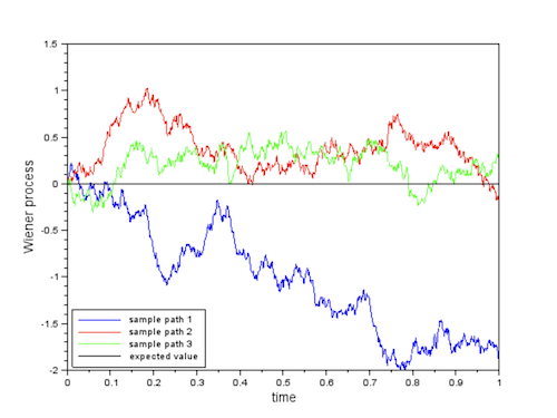
Figure: Three Possible Realizations of the Wiener Process
Three possible sample paths for the Wiener Process are shown above. The fact that Wiener process has variance $t$ implies that it tends to move away further and further away from the origin in proportion to $\sqrt{t}$ as time passes. But at the same time its mean remains zero, which means that returns to the origin quite often, in fact infinitely many times if we let it run to infinity.
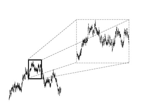
Figure: Self-Similarity or Fractal Property of the Wiener Process
The Wiener Process remains one of the weirdest objects that mathematicians have created, the idea of a continuous function not possessing a derivative at any point in its domain is highly non-intuitive. This is connected to another property of the Wiener Process, namely its self-similarity. This means that if we had a very powerful microscope and focused it on a tiny interval of time, what we would see would be indistinguishable from the larger picture of the Wiener Process. We can go on increasing the magnification, without ever encountering a limit to this property. Mathematically speaking, this property arises due to the fact that the random variables $W_t$ and ${1\over\sqrt{c}}W_{t\over c}$ possess the same distribution.
The mystery of the Wiener Process is due to the fact that it is defined over the continuum, which is like an endless pit, we can never get to the bottom of it. The Wiener Process performs its minuscule movements in the nooks and crannies of this pit, and this is something that is difficult to visualize at the macro level. And we can never get to the point where we can actually see the Wiener particle make its jumps, as we delve deeper, we continue to a continuous function with its craggy shape. This reminds me of another deep mystery from the science of Quantum Mechanics, the fact that we can never see a quantum particle like the electron in the act of moving, all we can see are discrete points in space which mark its path. In between those points, the electron travels in a mysterious realm in which it becomes a diffuse wave like phenomenon. This point is discussed further in my article Zeno’s Paradox of the Arrow. There is a relation between the Schrodinger equation and the equations of the Wiener Process that we will return at the end of this article.
There are a few important properties of the Wiener Process that I want to mention before we move on to the Ito Integral:
Uniqueness of the Wiener Process
The statement of the result is as follows: Let $X(t)$ be Random Process that satisfies the following two conditions:
- The Random Process is continuous, and
- It has Independent Stationary Increments Then there exist unique constants $b$ and $\sigma$, such that $X(t)$ is given by
Note that $X(t)$ is simply a scaled version of the Wiener Process, known as the Wiener Process with drift. It starts at $X(0)$ and is such that at time $t$, $X_t$ is distributed according to the Normal distribution $N(b,\sigma^2)$. Hence the Wiener Process can be considered to be an universal continuous time random process, since as soon as we constrain the increments to be ISI, there is only one process that can satisfy the two requirements. If we come across a continuous random process that is not Wiener, then either it won’t have the ISI property, or if it has the ISI property then it won’t be continuous. There are important continuous random processes, such as the Poisson Process, that fall in the latter category.
The uniqueness property can be understood using the following heuristic argument. From the continuity property we can write the increment $X_t - X_s$ as the sum of equal size smaller increments by sub-dividing the interval $[s,t]$, so that
\[X_t - X_s = \sum (X_{t_i} - X_{t_j})\]But the Independent Stationary Increment Property states that $(X_{t_i} - X_{t_j})$ are independent identically distributed random variables, so this equation is just a random sum. By the Central Limit Theorem, as the number of sub-divisions increases it follows that $X_t - X_s$ follows the statistics of a Normal distribution with variance $t-s$, i,.e., a Wiener Process. Note that because of the nature of the continuum, this sub-division is valid, no matter how small the interval $t-s$ is.
The Wiener Process is nowhere differentiable
I am not going to prove this here, but you can get some intuition why this is the case by considering the following equation
\[f(t) = f(s) + (t-s)f'(r)\]This is called the Mean Value Theorem in Calculus, and it says that it is possible to predict the value of a function at some future time $t$, based on its value at a past time $s$, and the derivative of the function at some $r$ that lies between $s$ and $t$. This clearly violates the ISI property of the Weiner process, since knowing $W(s)$ does not give us any information about the value of $W(t)$ in the future, however close $t$ maybe from $s$. From this we can conclude that the derivative $f’$ does not exist at any time $r$ in the rage $[s,t]$. The lack of derivative can also be deduced from the fact that $W(t)$ is a fractal curve. In order for the derivative to exist, the ratio ${W(t)-W(s)\over{t-s}}$ has to converge as $t$ gets closer and closer to $s$. Because of its fractal nature, $W(t)$ continues to move around randomly irrespective of how close $t$ is to $s$, thus ruling out the existence of this limit, and hence the derivative.
The lack of derivative again harks back to Zeno’s Paradox of the Arrow, which tries to prove that an arrow in flight is moving and not moving at the same time. Wierstrass was able to resolve this paradox by rigorously defining the velocity of the arrow, which is the same as defining the derivative ${dx\over dt}$. According to Wierstrass, even if the arrow is not moving at any one time instant, it still has a well defined velocity and hence moves over time. What if we replace the arrow by a particle moving according to the Wiener Process? In this case it does not have a derivative anywhere, so its velocity is not well defined. Then how does it still move, Wierstrass’s solution to the paradox does not apply anymore. Perhaps one way to look at it is that a physical particle such as a pollen grain always moves a finite amount before it changes direction, so it does have a well defined velocity. This means that a particle strictly moving according to the Wiener process is not physically realizable. The Wiener process is a mathematical idealization that captures extreme randomness, and is a popular modeling tool since it has nice analytic properties.
Quadratic Variation and Bounded Variation of the Wiener Process
The quadratic variation of a function $f$ on the interval $[a,b]$ over some partition $\Pi={a=x_0,x_1,…x_n=b}$ is defined as the limit
\[Q(f) = \lim_{|\Pi|\rightarrow 0} |f(x_i) - f(x_{i-1})|^2\]where $\Pi$ is the max value over the partitions $x_i - x_{i-1}$. Similarly the variation for $f$ is defined as the limit
\[V(f) = \lim_{|\Pi|\rightarrow 0} |f(x_i) - f(x_{i-1})|\]For regular functions, their variation is bounded, while their quadratic variation is 0. However, for Wiener Processes it can be shown that its variation diverges to infinity, while its quadratic variation over an interval $[a,b]$ is given by $b-a$. This means that
\[\lim_{n\rightarrow\infty}\sum_{i=1}^n |W_{kt/n} - W_{(k-1)t/n}|^2 = t\]Hence the squared difference of the values of a Wiener Process on an interval is just the length of the interval. This result is informally written as $(dW_t)^2 = dt$ and is critical in proving some important properties for the Wiener Process. For a proof of this property please see the paper by Carlstein.
Stochastic Calculus and the Ito Integral
Now that we have defined the Wiener Process, the next natural step is build upon this and create other random processes that use it as a building block. Kiyosi Ito carried out this program in the 1940s, and he started by defining a random process $I(t)$ that could be expressed as an integral over the Wiener Process:
\[I(t) = \int_0^t f(s,W_s) dW_s\]where $W(t)$ is a Wiener Process starting at the origin and $f(t,W_t)$ is another random process defined in terms of $W(t)$. Integrating with respect to a wildly varying random function is highly non-intuitive, how did he come up with this idea? It turns out that this integral arises naturally when we add a random noise component to a deterministic dynamical system model, such as the following one,
\[{dX(t)\over dt} = b(t,X_t)\]where $b$ is some function. Suppose that the time evolution of $X(t)$ has a random component that we want to capture. One way of doing this is by
\[{dX(t)\over dt} = b(t,X_t) + \sigma(t, X_t)N_t\]where $\sigma$ is another function and $N(t)$ is some sort of random process that models noise. Based on models used in engineering, we would like the random variables $N_{t_1}$ and $N_{t_2}$ to be independent, $E(N_t) = 0$ for all $t$, and require $N(t)$ to be a stationary process. This agrees with the intuitive notion that $X(t)$ is being driven by random noise impulses that can be completely different from one instant to another.
It turns out that there is no ‘reasonable’ process $N(t)$ that satisfies these conditions. In fact any such process would not even be continuous since we are requiring two neighboring random variables to be independent irrespective of how close they are in time.
Consider the discrete time version of this equation, that can be written as
\[X_k - X_{k-1} = b(t_k, X_k)\Delta t_k + \sigma(t_k,X_k)N_k\Delta t_k\]where $X_j = X(t_j), N_k = N(t_k)$ and $\Delta t_k = t_k - t_{k-1}$. Lets replace $N_k\Delta t_k$ by the increment of some stochastic process $V(t)$ such that $\Delta V_k = V_k - V_{k-1}$. Based on the properties of $N(t)$, we would like $V(t)$ to have independent stationary increments with mean 0, and lets also constrain it to be continuous. We learnt in the prior section that the only continuous random process with independent stationary increments is the Wiener Process so that the equation can be written as
\[X_k - X_{k-1} = b(t_k, X_k)\Delta t_k + \sigma(t_k,X_k)(W_k - W_{k-1})\]which is the same as
\[X_k = X_0 + \sum_{j=1}^k b(t_j,x_j)\Delta t_j + \sum_{j=1}^k \sigma(t_j,X_j)\Delta W_j\]Assume that the following limit exists as $\Delta t_j\rightarrow 0$,
\[X(t) = X_0 + \int_0^t b(s,X_s)ds + \int_0^t \sigma(s,X_s)dW_t\]and we can see the Ito Integral appearing on the right hand side of this equation. Note that $X(t)$ is now a random process, and so are $b$ and $\sigma$ since they are functions of $X(t)$ so that there are three sources of randomness in this equation. $b(t,X_t)$ is called the random drift of the Diffusion Process and $\sigma(t,X_t)$ is called the volatility.
This equation is often written in the differential form as
\[dX_t = b(t,X_t)dt + \sigma(t,X_t)dW_t\]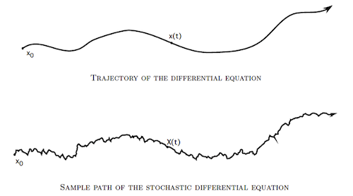
Figure: Diffusion Process of the type described by a Stochastic Differential Equation
Note that this is just an abbreviation of the integral form since $dX_t$, $dW_t$ and $dt$ don’t have any meaning by themselves. This is referred to as a Stochastic Differential Equation or SDE and the resulting process $X(t)$ is called a Diffusion Process. Tha latter name arises out of the observation that the equation describes the gradual spreading of a particle’s trajectory around the deterministic trajectory defined by ${dX(t)\over dt} = b(t,X_t)$, as shown in the above figure.
Does the Ito Integral even exist, in other words is it well defined? The traditional Riemann Integral is defined as the limit
\[\int_0^t f(t)dt = \lim_{n\rightarrow\infty}\sum_{i=1}^n f(t_i^q)(t_i - t_{i-1}),\ \ \ t_{i-1}\le t_i^q\le t_i\]where the sum is taken over the partition ${t_0 = 0, t_1, t_2,…,t_n = t}$. Clearly this won’t work since the Ito integral is not with respect to the time parameter. The Riemann-Stieltjes Integral on the other hand can be used to integrate with respect to another function, and is defined as:
\[\int_0^t f(t)dg(t) = \lim_{n\rightarrow\infty}\sum_{i=1}^n f(t_i^q)(g(t_i) - g(t_{i-1})),\ \ \ t_{i-1}\le t_i^q\le t_i\]This integral exists only if $g(t)$ has a bounded variation, i.e.,
\[V(g) = \lim_{|\Pi|\rightarrow 0} |g(t_i) - g(t_{i-1})|\]is a finite quantity. We saw in the last section that this property is not true for the Wiener Proces, hence we cannot use the Stieltjes Integral to define the Ito Integral.
We learnt about the concept of convergence in distribution in the prior sections, I am going to introduce another kind of convergence called convergence in probability which is needed to define the Ito Integral. A sequence of random variables ${X_t^n}$ is said to converge in probability to a random variable $X$, if for any $\epsilon > 0$,
\[\lim_{n\rightarrow\infty} P(|X_t^n - X|>\epsilon) = 0\]There is an useful result due to the Russian Mathematician Pafnuty Tchebychev which states that for a random variable $V$ with mean ${\overline V}$ and variance $\sigma_V^2$, for any $\epsilon > 0$
\[P(|V - {\overline V}|\ge\epsilon) \le {\sigma_V^2\over\epsilon^2}\]For random variable with zero mean, this becomes
\[P(|V|\ge\epsilon) \le {E[V]^2\over\epsilon^2}\]Hence given a sequence ${X^n_t}$ with mean 0, if we can show that $E(X^n_t - X_t)^2$ tends to zero as $n\rightarrow\infty$, then ${X^n_t}$ converges in probability to $X_t$. This is precisely how the existence of the Ito Integral is proven, by showing that it is the limit in probability of a sequence of simpler integrals.
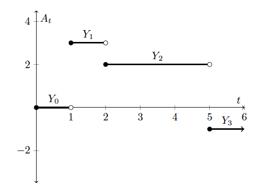
Figure: A Simple Integrand $A(t)$
Consider a simple random process $A(t)$ of the type shown in the above figure. It is constructed by choosing a finite number of time instants $0=t_0<t_1<…<t_n<\infty$ and associate a random variable $Y_j$ such that $A(t)= Y_j$ on the interval $t_j<t<t_{j+1}$. Furthermore he also assumed that the random variable $Y_j$ is independent of the further evolution of $W(t)$ for $t\ge t_j$. Random functions $A(t)$ that satisfy this property are referred to as $F_t$ measurable with respect to the Wiener Process. Then the stochastic integral for $A(t)$ is defined as
\[\int_0^t A(t)dW(t) = \sum_{i=0}^j Y_i(W_{t_1+1} - W_{t_i}) +Y_j(B_t - B_{t_j})\]Ito showed that if $A(t)$ is $F_t$ measurable then this integral satisfies the Ito Isometry property, which states that
\[E[\int_0^t A(s)dW(s)]^2 = \int_0^t E[A(s)^2] ds\]In the next step we will generalize the stochastic integral from simple processes to more general processes. It can be shown that it is always possible to approximate a bounded $F_t$ measurable process with continuous paths $A(t)$, as the limit of a sequence of simple processes $A^n(t)$, in the following sense:
\[\lim_{n\rightarrow\infty}\int_0^t E[A(s) - A^n(s)]^2 ds = 0, \ \ \ for\ \ \ all\ \ \ t\]From the Ito Isometry property it follows that
\[\lim_{n\rightarrow\infty}E[\int_0^t (A(s) - A^n(s)) dW(s)]^2 = 0, \ \ \ for\ \ \ all\ \ \ t\]An application of the Tchebychev inequality leads to the conclusion that $\int_0^t A^n(s)dW(s)$ converges in probability to $\int_0^t A(s)dW(s)$ as $n\rightarrow\infty$.
The Ito Integral allows us to build a wide variety of random processes by using the equation
\[X(t) = X_0 + \int_0^t b(s,X(s))ds + \int_0^t \sigma(s,X(s))dW(t)\]The analysis of the general case is not simple, however there are some simple special cases that occur frequently in applications:
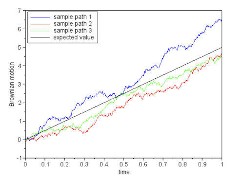
Figure: Three possible realizations of a Wiener Process with Constant Drift
- Weiner Process with Drift: This is given by the equation
In this case the SDE can be solved to obtain
\[X_t = X_0 + bt + \sigma W_t\]Hence this is a modified Wiener Process whose mean value increases linearly with time, and whose variance at time $t$ is given by $\sigma^2 t$. Its probability distribution at time $t$ is given by the Normal Distribution $N(X_0+bt, \sigma^2 t)$. Some example sample paths of a Wiener Process with drift are shown in the above figure.
- Time Homogeneuous Ito Diffusions: These follow the diffusion equation
Hence the dependence of $b$ and $\sigma$ on time is entirely captured by their $X_t$ dependence. Ito diffusions were a focus of research activity in the 1950s and 1960s, and their theory is well developed. An important property is that they are Markov Processes, just like the Wiener Process.
How does one go about solving a Stochastic Differential Equation? In the next section we will meet Ito’s Formula that allows us to get explicit solutions for some special cases, but there is a more general method which ‘solves’ these equations by simulating their sample paths, its called the Euler-Maruyama method. Its based on discretizing time in the interval $[0,T]$ into $n$ steps $[0, s, 2s,3s,…,Ns]$ such that $Ns=T$ and then carrying out the iteration
\[X_{(n+1)s} = X_{ns} + sb(ns,X_{ns}) + \sigma(ns,X_{ns})\sqrt{s}\epsilon\ \ \ n = 0,1,...,N-1\]where $\epsilon$ is a sample from the Normal distribution $N(0,I)$. Every time we run this iteration we, get a different sample path, and if we are interested in the average value or variance of $X_t$, then we can run multiple of these iterations starting from the same point $X_0$, and then take the average of the result.
The Ito Formula
In addition to defining his eponymous integral, Kiyoshi Ito made another fundamental contribution the field of Stochastic Calculus by discovering the Ito Formula (sometimes called Ito’s Lemma), which was published in 1951. It is the Differential Calculus counterpart to the Ito Integral, and can be considered to be a mathematical machine for transforming a given diffusion process into another. By use of this formula we can take a complex diffusion and transform it into a simpler diffusion, which is one of its common uses. It can also be used to compute the Ito Integral for some special cases, an example of which is given later in this section.
The Ito formula is a generalization of the Fundamental Theorem of Calculus as applied to stochastic integrals. Recall that the Fundamental Theorem establishes differentiation and integration as inverse operations, as follows
\[f(x) - f(x_0) = \int_x^{x_0} {df\over dx} dx\]Instead, what if the function $f$ operates on a Wiener Process instead, as in $f(W_t)$? Ito showed that the Fundamental Theorem has to be modifies as follows
\[f(W_t) - f(W_0) = {1\over 2}\int_0^t {\partial^2 f\over{\partial x^2}}ds + \int_0^t {\partial f\over{\partial x}} dW_s\]This equation can also be interpreted as stating that a function $f$ of the Wiener Process $W_t$ is a Diffusion Process with drift and volatility co-efficients given by ${1\over 2}{\partial^2 f\over{\partial x^2}}$ and ${\partial f\over{\partial x}}$. This is probably the most important result in Stochastic Calculus, it allows us to construct new diffusion processes from existing ones by operating on them using a suitable function $f$. For example if $f(x) = x^2$, then ${\partial f\over{\partial x}}=2x$ and ${\partial^2 f\over{\partial x^2}}=2$, thus
\[W_t^2 = \int_0^t 2W_s dW_s + {1\over 2}\int_0^t 2ds = 2\int_0^t W_s dW_s + t\]which allows us to compute the Ito Integral given by
\[\int_0^t W_s dW_s = {W_t^2 - t\over 2}\]Not that if this were an ordinary integral than the $-{t\over 2}$ term would not exist.
What if $f(t,X_t)$ is a function of a general diffusion process $X(t)$ given by $dX_t = b(t,X_t)dt + \sigma(t,X_t)dW_t)$? There is a generalized version of the Ito Formula that applies to this case, given by
\[f(t,X_t) - f(0,X_0) = {1\over 2}\int_0^t {\partial^2 f\over{\partial x^2}}(dX_s)^2 + \int_0^t {\partial f\over{\partial x}} dX_s + \int_0^t {\partial f\over{\partial t}} ds\]which can also be written as
\[f(t,X_t) - f(0,X_0) = \int_0^t ({\partial f\over{\partial s}} + b{\partial f\over{\partial x}} + {\sigma^2\over 2}{\partial^2 f\over{\partial x^2}} )ds + \int_0^t \sigma{\partial f\over{\partial x}} dW_s\]Hence the transformed process $f(t,X_t)$ is also a diffusion process with drift and volatility components as given above.
For example, if
\[Y(t) = X^2(t) + t^2\ \ \ where\ \ \ dX_t = b(t)dt + \sigma(t)dW_t\]then
\[dY_t = (2t + \sigma^2(t) + 2b(t)X_t dt + 2\sigma(t) X_t dW_t\]As an example of the application of Ito’s Formula, consider the following diffusion process which is used to model stock market returns (this model is discussed in detail in the next section):
\[dS_t = bS_t dt + \sigma S_t dW_t\]where $b,\sigma$ are constants. Does there exist a function $f$ such that $f(S)$ is a simpler diffusion process? Lets try the log function
\[f(S) = \log S\]Applying Ito’s formula it follows that
\[d(\log S) = bS{df\over dS}dS + {1\over 2}\sigma^2S^2{d^2f\over dS^2}dt + \sigma S {df\over dS} dW_t = (b - {\sigma^2\over 2})dt + \sigma dW_t\]Thus $\log S$ is a simple Wiener process with drift. Since the co-efficients $b,\sigma$ are constant, we can solve this equation to get
\[\log S(t) - \log S(0) = (b - {\sigma^2\over 2})t + \sigma W(t)\]which can be written
\[S(t) = S(0)\exp^{(b-{\sigma^2\over 2})t+\sigma W(t)}\]$S(t)$ is an important random process and is called the Geometric Brownian Motion.
Here is an informal proof of the Ito Formula:
The Taylor Expansion of $df(t,X_t)$, where $dX_t = b(t,X_t)dt + \sigma(t,X_t)dW_t$ can be written as
\[df(t,X_t) = {\partial f\over\partial t}dt + {\partial f\over\partial x} dX_t + {1\over 2} {\partial^2 f\over\partial^2 x} (dX_t)^2 + \ \ \ higher\ \ \ order\ \ \ terms\] \[= {\partial f\over\partial t}dt + {\partial f\over\partial x}(b.dt + \sigma.dW_t) + {1\over 2} {\partial^2 f\over{\partial^2 x}}[(b^2.(dt)^2 + 2b.\sigma.dt.dw_t + \sigma^2.(dW_t)^2] + \ \ \ higher\ \ \ order\ \ \ terms\]From the prior section we saw that the Quadratic Variation Property for Wiener processes imples that $dW_t^2 = dt$, while the terms with $dt^2$ and $dt.dW_t$ can be ignored. Also ignoring the higher order terms we get
\[df(t,X_t) = [{\partial f\over\partial t} + b.{\partial f\over\partial x} + {\sigma^2\over 2}{\partial^2 f\over{\partial^2 x}}]dt + {\partial f\over\partial x}.\sigma.dW_t\]which is the Ito Formula.
Modeling the Stock Market
When I first learnt about the Wiener Process and Stochastic Calculus in grad school in the late 1980s, the main applications that text books talked about were in the fields of filtering and control theory. Now 40 years later almost everyone who learns Stochastic Calculus is doing it so that they can apply it to mathematical finance, in other words, to become a Wall Street quant. In 1985 the Black Scholes equation was already about a decade old, but its use hadn’t become prevalent in Wall Street. There has been an explosion in the financial markets since then, with new financial products that make use of stock derivatives and this has made Stochastic Calculus a must have skill for quants. At the same time there has been a backlash against the use of the Wiener Process to model stocks, especially after the 2007-2008 financial crisis. A prominent voice arguing for this is the trader and author Nassim Nicholas Taleb though some of these ideas can be traced back to a paper that Benoit Mandelbrot wrote on this topic in the early 1960s.
The stock market is the closest anyone of us will get to encountering pure randomness in our daily lives. Understanding how the market behaves is important to most of us who have part of our savings invested in the market, but we normally don’t think about it unless at times of market turmoil. However there is a class of financial industry professionals called equity traders who have to deal with this randomness on a day-to-day basis. They buy and sell equities frequently, sometimes several times a day, and their profession is a constant struggle against the randomness of the market.
The earliest random process model for stocks can be traced back to Bachelier from his PhD thesis back in 1901. It uses a Wiener Process with drift given by (though it was not called by this name then)
\[S(t) = \mu dt + \sigma W(t)\]The first term captures that fact that there is usually an upward drift in the market over time, while the second term captures the volatility in the process. Since the Wiener process has independent and stationary increments, it implies that the random change $S_{t+h} - S_t$ in $S(t)$ is independent of whatever happened in the market at time $t$ and earlier, including the value $S_t$ as well. This does not agree with the way the stock market actually behaves, since in reality the change is greater if $S_t$ is larger. In the 1960s Samuelson improved the model by noting that the change in the value of a stock is dependent on its current price, since only the percentage increase or decrease from the current price is what really matters to a trader. In other words, it doesn’t matter whether you are holding a million dollar portfolio or a one dollar portfolio, you would still want the same 10% annual return. Taking this into account, the modified model is
\[dS_t = \mu S dt + \sigma S dW_t\]which states that the fractional change ${dS_t\over S}$ should be a Wiener Process with drift.
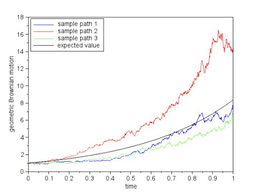
Figure: Three Possible Realizations of the Geometric Wiener Process
As shown in the prior section, this Stochastic Differential Equation can be solved using the Ito Formula to obtain
\[S(t) = S(0)\exp^{(\mu-{\sigma^2\over 2})t+\sigma W(t)}\]This is known as the Geometric Wiener Process, and is the most common stock market model used today. Since all changes are in terms of percentage increments or decrements, this means that the value of $S(t)$ can never dip below zero, unlike the plain Wiener Process with drift. If there was no random component, $S(t)$ will evolve as
\[S(t) = S(0)\exp^{\mu t}\]This equation says that when the volatility is zero, the stock price grows at a continuously compounded rate of $\mu$ per unit time. The Geometric Wiener Process can be regarded as a random variation around this exponential curve. The above figure shows three possible sample paths of the Geometric Wiener Process, along with the deterministic curve.
Note that the Geometric Wiener Process does not have the Independent Stationary Increment property, since the increment $S_{t+h} - S_t$ is dependent on the starting value $S_t$. It is still a Markov process though and its logarithm can be written as
\[\log S(t) = \log S(0) + (\mu - {\sigma^2\over 2})t +\sigma W(t)\]which is just the standard Wiener Process with drift.
Bachelier’s original market model of the Wiener Process with drift can be regarded as the value of an investment in which the gains are not invested back into the portfolio, hence any change is due to gain or loss in the starting amount $S(0)$. The model based on the Geometric Wiener Process on the other hand re-invests its gains back into the portfolio, so it results in the exponential behavior due to continuously compounding gains.
This model is based on the assumption that the future of the stock market cannot be predicted by the knowledge of how it has done in the past, only the current price matters, which is same as the Markov property. This is also known as the weak form of the Efficient Market Hypothesis (EMH) in finance, and was most forcefully advocated by the economist Eugene Fama in the late 1960s. There is a group of investors known as Technical Analysts who try to predict the market by looking at stock patterns that have occurred in the past, thus directly contradicting the EMH. This is an extremely difficult undertaking, and most Technical Analysts end up loosing money. However there are a few that do manage to beat the market, at least during intervals, and this raises the question of whether the market behavior varies over time, so that there are times when the EMH is violated.
Does the Stock Market Follow a Wiener Process?
Wiener Process models for the stock market have been used since the 1960s, after Samuelson introduced Bachelier’s original work to the financial community. A huge amount of money, trillions of dollars, is tied to trades that base their justification on this model. In particular the Black-Scholes model for option’s pricing, probably the most important formula in use in financial markets, is based on the Wiener Process model. The question arises: Are we justified in using the Wiener Process to model the market?
Assume that the stock price closed at $S(0)$ at the end of the previous trading day, then by using the Euler-Maruyama method for simulating a SDE, the model says that the price at the end of the next trading day is distributed according to the random variable $S_t$ given by
\[\log S_t = \log S_0 + (\mu - {\sigma^2\over 2})t +\sigma \sqrt{t}\epsilon\]where $\epsilon$ is a sample from a Normal (or Gaussian) Distribution with mean $0$ and variance $1$. This random variable is independent of anything that might have happened in the market on the previous day, or any of the days before that. Paul Samuelson justified this model by stating that all the information needed to trade on day $n+1$ is entirely summarized by the price of the stock at the end of trading day $n$, i.e., the EMH. Hence any change in the value of the stock that happens on day $n+1$ is due to new information that comes in as the day progresses, and any such information is instantly incorporated into the price of the stock. This makes the assumption that all traders have access to most complete information that is available about factors that affect the market at all times, and moreover they are all perfectly rational humans who are able to make trading decisions using the facts as they become available.
Samuelson’s assumptions justifying the use of the Wiener Process model have been disputed over the years since it was first proposed. One large contingent whose entire profession is based on the proposition that the EMH is not true, is the Hedge Fund industry. Most of them place their trades on the basis of their understanding of how the market will behave based on various factors in the past history. The best Hedge Funds, such as Renaissance Capital, have consistently beaten the market over a time period of decades, which makes one think that they have discovered some regularities in the market, and this goes against the EMH. The economists Sanford Grossman and Joseph Stiglitz gave the following argument against the EMH: All trading is based on two parties getting together and coming to an agreement on the price of a stock The buying party believes that the stock will appreciate, while the selling party has the opposite view. In order to make this trade happen, each party has presumably done some research to justify their actions, and this research is usually based on the past history of the stock, the industry it is in, the state of the economy etc. However if the EMH were true, all this research would be completely useless, since everything that there is to know about a stock is summarized in its current price. Thus all trading on Wall Street would grind to a halt.
A lot of work in this area has been done by Professors Andrew Lo and Craig Mackinlay, who teach at MIT and UPenn respectively. Lo has written a nice book on this topic for the general public called Adaptive Markets where his ideas are lucidly explained. For those wanting to dig deeper into the math and statistics they used in their work, can read their book A Non-Random Walk Down Wall Street. Lo and Mackinlay argue that Samuelson’s assumptions that all trader’s are perfectly rational people, who at any instant have all the information needed to trade the stock they are interested in, is not quite true in the real world. Most traders don’t make use of all the the available information to make their decisions, they use partial information and heuristics instead, which is known as the Bounded Rationality hypothesis. Moreover not all traders are at the same level of expertise. There are the Wall Street quants who are experts at their jobs, and then there is the mass of mom and pop traders who trade on the basis of what they last heard on TV, and this creates opportunities for profits to flow in the expected direction. In their opinion the EMH may be approximately true if the market has reached an equilibrium, where there is very little volatility so that the trading heuristics that traders use work most of the time. But at times of extreme market volatility, such as what happened during the 2007-2008 Financial Crisis, the trading environment changes radically, and the old rules go out of the window. During these times the EMH certainly does not hold, and it creates an opportunity for the savviest of traders who manage to keep their heads amid the turmoil.
Lo and Mackinlay carried out statistical tests on the market data to see whether it satisfies the assumption of a Wiener Process. They did two kinds of tests:
-
If the random variable $\log S_t - \log S_0$ were indeed distributed according to the Normal distribution $N(\mu, \sigma^2 t)$, then its variance over a time period $t$ should be proportional to $t$. Lo and Mackinlay found that the variance of two-week returns was three times the variance of one week returns, not twice the variance as the theory predicts. In other words the variance varies as $1.5t$ as a function of time, rather than $t$, which means the market increments do not follow the Normal distribution.
-
Lo and MacKinlay also tested the applicability of the independent stationary increments property to the market by computing the 750-day rolling-window first-order autocorrelations over successive days for the market index, over the period from 1928 to 2013. An autocorrelation of 1 implies that that tomorrows market return will be positive (or negative) if it was positive (or negative) today, a value of -1 implies that the market will flip in the successive days from positive to negative or vice-versa while a value of 0 implies that the market returns on successive days are independent, i,e, the EMH. Their result is plotted on page 281 of Adaptive Markets. It shows that there were only two periods in which the autocorrelation was close to zero, during the 1930s, and in the period from the mid 1980s to the end of the millennium. In the period from the 1940s to the mid 1980s, the autocorrelation was consistently positive, in other words there was a lot of money that could have been made by betting the market will behave tomorrow as it did today. Since the early 2000s on the other hand, the autocorrelation has become negative, i.e., the market reverses itself on most days. In any case, this shows that the independent stationary increments property is rarely true for the market.
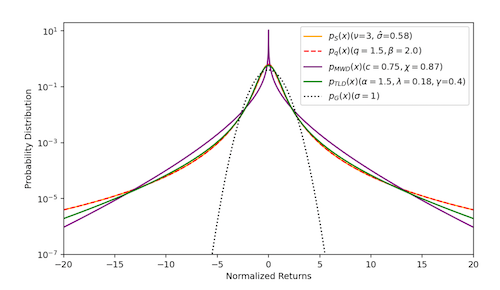
Figure: Comparison of the Normal Distribution with Fat Tailed distributions
So if the market does not follow the Wiener Process, what kind of statistics best describe it? The most straightforward way of approaching this problem is by empirically estimating the distribution of $\log S_t$, i.e. the log of the market gains in an interval $t$. As shown in the above figure, this distribution is distinctly non-Normal (the Normal distribution has also been plotted using the dotted line). It typically exhibits a sharp central body and a fat-tailed behavior, which leads to large price movements. This means that extreme events occur more often than predicted by the Normal distribution.
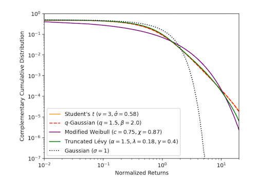
Figure: Tail Behavior comparison of the Normal and Fat Tailed distributions
The empirical returns in the tails behave as a power law $p(x)\propto {1\over{\vert x\vert^{1+\alpha}}}$ with the exponent $\alpha$ close to 3 in the limit, which is further illustrated in the plot of the complementary distribution function $\int_x^\infty p(x)dx$ as shown above. There are a number of distributions that obey the power law, the most popular being the Truncated Levy Distribution (TLD).
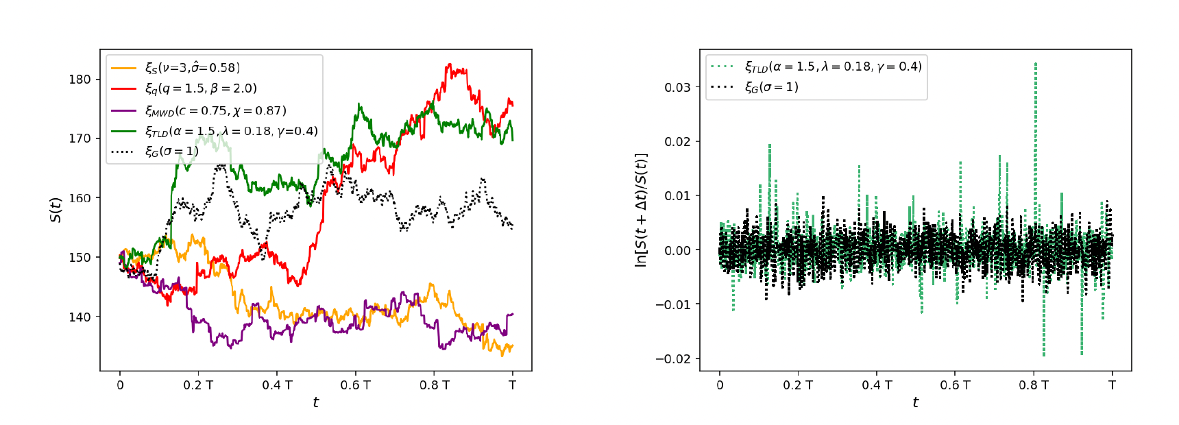
Figure: Sample Paths generated by Fat Tailed Distributions (left) and the sample log returns for the Normal and the Truncated Levy distributions (TLD)
We can plot the sample paths for a random process following the non-Normal distributions by using a slightly modified form of the Euler-Maruyama equation to generate samples at intervals of $t$
\[\log S_t = \log S_0 + (\mu - {\sigma^2\over 2})t +\sigma \sqrt{t}\xi_{NG}\]Here $\xi_{NG}$ is a sample drawn from a Non-Normal distribution with mean $0$ and variance $1$. This equation implicitly assumes that successive samples for non-overlapping intervals are independent, and also that the variation with $t$ follows the $\sqrt t$ property of the Wiener Process. The left hand side plot in the above figure shows the results of the simulation, and we can see that non-Normal processes exhibit large jumps from time to time which has a greater resemblance to the actual behavior of financial markets. This is further illustrated in the right hand side plot, which plots samples of the log return ($\log S_t - \log S_0$) for the Normal and the Truncated Levy distribution.
Earlier in this article I stated that the Wiener Process with drift enjoys the uniqueness property, i.e., it is the only random process which is continuous with independent stationary increments. This seems to contradict the above figure which shows the simulation of other random processes, such as the Truncated Levy, which have these properties. As you may have guessed, the resolution to this contradiction lies in the fact that the non-Normal sample paths shown in the figure are not continuous, since there is always a finite time difference between successive changes in $S_t$ in the simulation. However, even in this case, as $t$ becomes larger, $S_t$ can be written as the scaled sum of independent identically distributed random variables, which tends towards a Normal distribution because of the Central Limit Theorem. Hence for large values of $t$, we can expect the non-Normal processes to converge to the Wiener Process with drift.
The most important application of the Wiener Process model in finance is the Black-Scholes equation for options pricing, which is given by
\[rf_t = {\partial f_t\over\partial t} + rS_t {\partial f_t\over\partial S_t} + {\sigma^2 S_t^2\over 2}{\partial^2 f_t\over\partial S_t^2}\]In this equation, $f(S_t,t)$ is the value of a European style call option, $r$ is the constant risk-free rate of return, and $S_t$ is the stock on which the option is based. The model assumes that $S_t$ follows the Geometric Wiener Process model described earlier with variance $\sigma^2$. The model is independent of the value of the drift co-efficient $b$. Note that this is a regular Partial Differential Equation, not a SDE. I am not including a derivation of this equation, but if you are interested, an excellent description can be found in this article. The main tool used in the derivation is the Ito Formula, and it can be understood using the Stochastic Calculus concepts developed in this article.
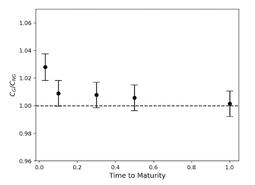
Figure: Prices of European Call Options as computed by the Black-Scholes model (dotted line) and the Truncated Levi Distribution (TLD) based model
What are the effects of a non-Wiener Process model on call options pricing? As shown by Domenico et.al., it is possible to price options using Monte Carlo simulations driven by sample paths of the random process controlling the market movements, and this is plotted in the above figure. It shows that there is big discrepancy between the Black-Scholes model and non-Normal models for small values of Time to Maturity for the option. However, as $t$ increases, these values converge, and this is due to the fact that the non-Normal random process converges to the Wiener Process as $t$ increases.
Image Generation using the Langevin Diffusion Process
Paul Langevin was a physicist who worked in Paris in the early decades of the 20th century. He proposed an improvement to Einstein’s model for Brownian Motion by using the following equation to model the motion of particles in a viscous fluid, which reads as follows (with the notation that $v(t)$ is the velocity of the particle at time $t$ and $m$ is its mass):
\[m dv_t = -\lambda v_t dt + \eta dW_t\]The first term on RHS of the equation represents the viscous force on the particle that dampens its movement while the second term represents the random forces due to collisions with the molecules of the fluid. One of the most unexpected applications of the Wiener Process happened in 2015 when Jascha Sohl-Dickstein and his collaborators showed that the Langevin Process can be used to generate images. Until then the best image generation technique was based on a type of Neural Network called Generative Adversarial Networks or GANs, which are notoriously difficult to train. It was shown within a few years that the diffusion based technique yielded better images, and could be extended to encompass text to image generation as well as video generation. This has led to widespread adoption of tools such Dall-E-2 and Dall-E-3 from OpenAI and Imagen from Google which are all based on this technique.
In order to understand the connection between diffusions and image generation, consider a typical digital image. It is made up hundreds of thousands of individual blobs of color called pixels, the value of which is represented by a group of three integers between 0 and 255, for the red, blue and green colors. For any one image the value of a pixel is fixed, but if we have a collection of images, then the pixel value varies and can be considered to be a random variable. The collection of $n$ pixels that make up an image can be considered to be a random vector $(X_1, X_2,…,X_n)$ consisting of correlated random variables, with probability distribution $f(x_1, x_2,…,x_n)$. If we had access to this distribution, then it would be possible to generate new images by sampling from it. In reality $f$ is some fantastically complex function which cannot be described using a simple equation. But what if we sample from a simpler distribution, such as the Normal distribution, and then somehow modify the samples so that they end up following $f$ instead? This can be accomplished by using the Langevin diffusion.
Consider the following n-dimensional Stochastic Differential Equation of the Langevin type
\[dX_t = \nabla\log p(X_t)dt + \sqrt{2} dW_t\]Note that $X(t) = (X_{1}(t), X_{2}(t),…,X_{n}(t))$ and $W(t) = (W_(t),W_2(t),…,W_n(t))$ are n-dimensional random processes, while $\nabla$ is the vector operator $\nabla = ({\partial\over {\partial x_1}}, {\partial\over {\partial x_2}},…,{\partial\over {\partial x_n}})$. Also $p(x_1,x_2,…,x_n)$ is the target probability density function that we are trying to move the distribution of $X_t$ to. This SDE can be simulated using the Euler-Maruyama technique, resulting in
\[X_{t+s} = X_t + s\ \log\nabla\log\ p(X_t) + \sqrt{2s}\epsilon\]In this equation $s$ is the step size and $\epsilon$ is a n-dimensional noise sample from the Normal distribution $N(0,I)$. This can be interpreted as an update to the value of $X_t$ by moving in the direction pointed to by $\nabla\log p(X_t)$, which is somewhat similar to the parameter update step in the Stochastic Gradient Descent Algorithm used for training Neural Networks, though in this case we are performing an ascent, not descent. The presence of the second term adds some random noise to the step update. Note that the gradient term pushes $X_t$ into regions where the value of $p(x)$ is high. Thus as $X_t$ evolves over time, it moves into regions with high probability, and in the limit it is distributed according to $p(x)$. But what about the noise term? It has been put there to prevent $X_t$ from getting stuck in a local maximum of $p(x)$, which would cause the iteration to get stuck and there would be no movement.
The Langevin diffusion gives us a very powerful tool for sampling from complex distributions, and we are going to use it to sample from the distribution of pixel values in images.
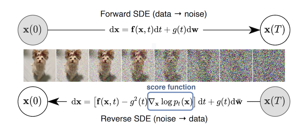
Figure: Using Stochastic Differential Equations to transform an image into noise (top, from left to right), and transforming noise back into an image (bottom, right to left)
The main idea behind using Stochastic Differential Equations to generate images is shown in the above figure, and consists of the following steps:
Forward Diffusion
We will treat the pixels of the image as the components of a n-dimensional random process $X(t)$, whose initial value $X(0)$ is equal to actual pixel values, and is distributed according to some unknown distribution given by $p_{data}(x_1,x_2,…,x_n)$. As shown in the arrow going from left to right in the top part of the figure, we now let $X(t)$ evolve according to the following Stochastic Differential Equation
\[dX_t = f(X_t,t)dt + g(t)dW_t\]so that at time $T$, the distribution of $X_T$ is given by $p_T(x_1,x_2,…,x_n)$. We choose the functions $f$ and $g$ such that $p_T(x_1,x_2,…,x_n)$ is distributed according to the Normal distribution $N(0,I)$ regardless of its initial distribution. As shown in the figure, the end result of this process is that the pixels get completely randomized, so that all correlations between them are lost, and the end result is a noise image.
Backward Diffusion
The Backward Diffusion allows us to sample from the original distribution $p_{data}(x_1,x_2,…,x_n)$, by sampling from the Normal distribition $N(0,I)$ at $t=T$ and then use the Langevin Diffusion to work backwards to recover $p_{data}(x_1,x_2,…,x_n)$ at $t=0$. In other words we start with pure noise, and gradually convert it back into a proper image. In order to do this we introduce a Reverse Time SDE given by
\[d{\overline X}_t = [f({\overline X}_t,t) - g^2(t)\nabla_x\log\ p_t({\overline X}_t)]dt + g(t)d{\overline W}_t\]where $p_t(x)$ is the distribution for $X_t$. In this equation time runs backwards from $t=T$ to $t=0$, and the Backwards Wiener Process ${\overline W_t}$ has the property that ${\overline W}_{t-s} - {\overline W}_t$ is independent of ${\overline W}_t$ for $s>0$. The mathematician Brian Anderson showed in the 1980s that the time reversed diffusion process ${\overline X}_t$ has the same distribution as the forward time process $X_t$.
Hence $X_T$ is sampled from a Normal distribution, and then its value is allowed to change according to this SDE. With appropriate choice of $f$ and $g$, this equation can be shown to be equivalent to the Langevin Diffusion Process. This implies that the noisy image $X_T$ with distribution $N(0,I)$ is gradually transformed into a proper image $X_0$ sampled from the distribution $p_{data}(x_1,x_2,…,x_n)$.
Song et.al. proposed the following choice for the functions $f$ and $g$,
\[f(x,t) = 0\ \ \ and\ \ \ g(t) = \beta'(t)\]where $\beta’(t) = {d\beta\over dt}$ is a function with the properties $\beta(0) = 0, \beta’(t) > 0, \beta(t)\rightarrow\infty$ for $t\rightarrow\infty$, which results in the Forward Diffusion
\[dX_t = \beta'(t) dW_t\]It can be shown that variance $V(X_t)$ satisfies the equation
\[V(X_t) = V(X_0) + \beta(t)\]so that it increases monotonically with $t$, which implies that $X_t$ divergesas $t$ increases. However the scaled process $Y_t = {X_t\over{\sqrt{\beta(t)}}}$ converges to the Standard Normal distribution $N(0,I)$.
For this choice of $f$ and $g$, the Backward Diffusion can be written as
\[d{\overline X}_t = -g^2(t)\nabla_x\log\ p_t({\overline X}_t)dt + g(t)d{\overline W}_t\]In practice these equations are implemented using the Euler-Maruyama method by discretizing time which results in a multistage process shown in the figure. In discrete time the Backward Diffusion equation becomes
\[{\overline X}_{t-s} \approx {\overline X}_t + sg^2(t)\nabla_x\log\ p_t({\overline X}_t) + g(t)\sqrt{s}\epsilon\]where $\epsilon$ is sampled from the Normal distribution $N(0,I)$. Recall that the Langevin Diffusion was given by
\[X_{t+h} = X_t + s\ \nabla\log\ p(X_t) + \sqrt{2s}\epsilon\]and it had the property that the distribution of $X_t$ converges to $p(X)$ over time. The Backwards Diffusion equation has the same struscture, with the difference that $p_t(x_1,x_2,…,x_n)$ is used rather than the target distribution $p_{data}(x_1,x_2,…,x_n)$. However $p_t(x_1,x_2,…,x_n)$ converges to $p_{data}(x_1,x_2,…,x_n)$ as $t\rightarrow 0$, so that the Langevin convergence still holds.
In the discussion so far the subject of Neural Networks has not come up, so what role do they play? The probability distribution over images $p_{data}(x_1,x_2,..,x_n)$ or $p_t(x_1,x_2,…,x_n)$ are so complex that they cannot be expressed in the usual way by using mathematical equations, and this goes for the gradient $\nabla\log p_{t}$ as well. However even the most complex distribution can be represented using the millions of parameters in a Neural Network, and this is something that has become possible only in the last decade as our ability to train these networks has improved. These networks can be trained to estimate $\nabla\log p_{t}$, lets call is $r(\theta, X_t,t)$, where $\theta$ represents the parameters of the Neural Network. With this substitution the equation for recovering the distribution $p_{data}(x_1,x_2,…x_n)$ becomes
\[{\overline X}_{t-s} \approx {\overline X}_t + sg^2(t) r({\theta},{\overline X}_t,t) + g(t)\sqrt{s}\epsilon\]The network is trained by minimizing the error between the images generated by the Backward Diffusion and the original images in the training dataset, and this process is repeated hundreds of thousands of times until the parameters converge.
The description that I just gave contains the essence of the argument about how diffusion based image generation systems work. If you want to dig deeper into this subject, including details about the implementation, you can read the excellent blog by Peter Holderreith on this topic or the original paper by Song et.al. I have also written a tutorial on this subject and it can be found here.
Is There a Connection with Quantum Mechanics?
I remarked at the start of this article that Quantum Mechanics and the Wiener Process were both birthed in the year 1900, but are they related? Considering that both of them involve the concept of randomness at a very deep level, one might suspect that to be the case. Quantum Mechanics is based on the concept of a Wave Function $\psi$, for which we still don’t have a physical interpretation. It gives no clear picture of the motion of particles in-between successive measurements and leads to predictions that are probabilities. But these probabilities enter the theory in a rather artificial way, through the Born Rule, which in one dimension states that the probability $p(\Delta x)$ of finding a particle in the interval $\Delta x$ is given by
\[p(\Delta x) = \int_{\Delta x} \psi\psi^* dx\]All of Quantum Mechanics is based on this rule, but again we have no clue as to why it works. It is not possible to write down an expression such as $x(t)$ to describes the path of a particle in Quantum Mechanics, all we can predict are the probabilities. In diffusion processes on the other hand, the location of a particle is also probabilistic, but unlike Quantum Mechanics, we do have Stochastic Differential Equations that explain how the probabilities get into the model.
Is it possible to introduce randomness into Quantum Mechanics without using the Born Rule? And more interestingly, can that randomness be due to the fluctuations of some sort of diffusion process operating at a very deep level in nature? Einstein showed that the randomness of the pollen particles was due to bombardment by water molecules. Is there some phenomenon operating deep in the structure of space-time that similarly causes randomness in Quantum Theory by randomly bombarding tiny particles such as the electron. If this were true, it would provide a physical explanation for mysterious equations of Quantum Mechanics that would have made Einstein happy!
There has been some work done over the years to connect Quantum Mechanics and the diffusion processes, and in order to understand this, I am going to introduce an important equation in the theory of diffusion processes called the Fokker-Planck equation. Consider the diffusion given by
\[dX_t = m(X_t, t)dt + \sigma^2(X_t, t)dW_t\]The Fokker-Planck equation for this diffusion is a Partial Differential Equation for the probability density $\rho(x,t)$ for the random variable $X_t$ and is given by
\[{\partial\rho(x,t)\over{\partial t}} = {1\over 2}{\partial^2\rho(x,t)\sigma^2(x,t)\over{\partial x^2}} - {\partial\rho(x,t)m(x,t)\over{\partial x}}\]Note that for the case of a Wiener Process, $m = 0$ and $\sigma = 1$, so it reduces to
\[{\partial\rho\over{\partial t}} = {1\over 2}{\partial^2\rho\over{\partial x^2}}\]which has the expected solution
\[\rho(x,t) = {1\over{\sqrt{2t}}} exp^{-{x^2\over{2t}}}\]In the case of Quantum Mechanics we have the Schrodinger Equation for $\psi$ given by (for the case when there are no external fields)
\[i{\hbar}{\partial\psi\over{\partial t}} = -{\hbar^2\over{2m}}{\partial^2\psi\over{\partial x^2}}\]Consider the motion of a particle in free space, which is initially localized in the neighborhood of the origin. Unlike for the Wiener Process, we cannot have the particle be located exactly at $x=0$ at $t=0$, since the Heisenberg Uncertainty Principle would require that it have an infinite uncertainty in its initial momentum. Instead we assume that its wave function at $t=0$ is distributed according to a Normal distribution given by (with $m = \hbar = 1$ and $\sigma^2 = {1\over 2}$),
\[\psi(x,0) = \sqrt[4]{2\over\pi} \exp^{-x^2 + ip_0x}\]where $p_0$ is the initial average momentum of the particle. Hence both the initial position and the initial momentum of the particle are Normally distributed random quantities, connected together by the Uncertainty Principle. Solving the Schrodinger equation will tell us how the particle’s location changes with time, and this results in the expression (see this article for a nice description of free quantum particles)
\[\psi(x,t) = \sqrt[4]{2\over\pi}{1\over\sqrt{1+2it}}\exp^{-{(x-p_0t)^2\over {1+4t^2}}} \exp^{i{(p_0+2tx)x-{tp_0^2\over 2}\over {1+4t^2}}}\]with probability density given by
\[|\psi(x,t)|^2 = \sqrt{2\over\pi}{1\over\sqrt{1+4t^2}} \exp^{-{(x-p_0t)^2\over {1+4t^2}}}\]For large values of $t$, this can be written as
\[|\psi(x,t)|^2 = {1\over\sqrt{2\pi t^2}} \exp^{-{2(x-p_0 t)^2\over {2t^2}}}\]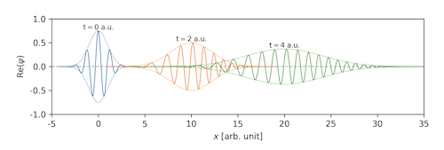
Figure: Probability distribution of a free particle as a function of time
This equation says that if the particle with initial average momentum $p_0$ is initially confined to a location around the origin at $t=0$, then on the average it moves to the right, but we can’t predict its exact location. The probability of locating it in a specific area is governed by a Normal distribution centered at $p_0 t$, i.e., on the average it has moved to the right, and its location has become even more uncertain due to the variance which increases as $t^2$ (see above figure).
The quantum mechanical explanation for this behavior is the following: Since the initial momentum is a random quantity, as time increases the range of possible distances covered by the particle increases depending on the spread of the momentum values, but there is no explanation for where the randomness is coming from. The expression does look suspiciously like the probability density for a Wiener Process with drift, except that variance has a $t^2$ dependence on time, rather than $t$. Hence the range of possible locations for both a Wiener particle and a quantum particle becomes more and more spread out over time.
Is it possible to come up with a diffusion process whose probability distribution behaves like the one predicted by the Born Rule? In other words, does the quantum particle derive its randomness from being driven by a Wiener Process? If so, this would be a natural way to introduce probability into Quantum Mechanics, rather than using the Born Rule. There have been various attempts over the years to solve this problem, including by Schrodinger himself, since he was not happy with the Born Rule interpretation for his wave function. The best known theory was proposed by Princeton mathematician Edward Nelson in the mid 1960s and goes by the name Stochastic Quantum Mechanics (see this article for a recent review of Nelson’s theory).
Nelson assumed that a quantum particle in free space is driven by the following Stochastic Differential Equation
\[dX_t = b(X_t,t)dt+ dW_t\]The function $b(X_t,t)$ is called the mean forward velocity, while $W(t)$ is a standard Wiener Process with mean zero and variance $\nu = {\sigma^2\over 2}$. Unlike the case for Brownian Motion, there is no fluid that is pushing the particles around, and Nelson left open the question of what is responsible for the randomness. He suggested it could be due to processes happpening deep in the fabric of space-time which we cannot detect. Markopoulou and Smolin have proposed a theory for the structure of space-time which also makes use of this idea.
The Fokker-Planck equation for the probability density for this diffusion is given by
\[{\partial\rho\over\partial t} = -{\partial(b\rho)\over\partial x} + \nu{\partial^2\rho\over{\partial x^2}}\]Nelson proposed the following special form for the diffusion trajectory of the particle
\[dx_t = [{1\over m}{\partial S(x,t)\over{\partial x}} + {\nu\over R^2(x,t)}{\partial^2 R^2(x,t)\over{\partial x^2}}]dt + dW_t\]where the functions $S(x,t)$ and $R(x,t)$ are constrained to satisfy the following equation
\[{\partial S(x,t)\over{\partial t}} = -{1\over{2m}} ({\partial S(x,t)\over{\partial x}})^2 - V + {\hbar^2\over{2mR(x,t)}} {\partial^2 R(x,t)\over{\partial x^2}}\]If we specify that the probability density for the diffusion be equal to $R^2$, i.e., $\rho = R^2$, then the Fokker-Planck equation simplifies to
\[{\partial R^2\over\partial t} = - {1\over m} {\partial{\partial S\over{\partial x}} R^2\over{\partial x}}\]These last two equations are called the Madelung equations, and can also be derived by setting $\psi = R\exp^{iS\over\hbar}$ in Schrodinger’s equation. This implies that diffusion model and the Schrodinger model for a quantum particle are equivalent descriptions, since the equations for both these models can be reduced to the Madelung equations. Hence the Schrodinger equation is just a convenient mathematical way to write the Madelung equations, it does not have any real existence in nature. But can we assume that the Schrodinger equation were not known, and then derive it by using the Madelung equations? This part of the theory does not quite work yet, and has prevented it from achieving greater prominence in the physics community.