Image Generation Using Diffusion Models
Introduction
One of the important applications of Neural Networks has been image generation. Given a set of training samples ${X_1,…,X_N}$, the preferred approach to generating a new datapoint $X = (x_1,…,x_n)$ is to first estimate the distribution $p_\theta(X)$ that approximates the actual distribution $p(X)$ that the training samples come from (using Unsupervised Learning) and then sample from $p_\theta(X)$ to generate a new $X$. There are several ways in which this program can be put into practice:
-
Autoregressive Generation: This technique works by building a model for the parametrized distribution $p_\theta(X)$ that maximizes the log likelihood of the observed data points ${X_1,…,X_N}$, and then generates new datapoint $X=(x_1,…,x_n)$ by making use of the recursion \(x_i = argmax_i\ p_\theta(x_i|x_1,...,x_{i-1})\) This technique is more commonly used in NLP applications, where the $p_\theta$ was implemented using a RNN/LSTM or Transformer. Images can also be generated by using this technique, using algorithms such as pixel-RNN or pixel-CNN. The main issue with using autoregressive image generation models is that they do generation on a pixel by pixel basis. Given a typical RGB image contains a few hundred thousand pixels, this can be a slow process.
-
Generative Adversarial Networks (GANs): A much improved way of generating images was discovered in 2014, by means of a class of DLNs called Generative Adversarial Networks or GANs. Instead of trying to maximize the log likelihood of a distribution function, GANs work by pairing the Generative Network (that generates the image in one shot as opposed to pixel by pixel) with another network called the Discriminator whose job is to identify real images from the training dataset from those generated by the Generator. As the Discriminator becomes better at its job, the Generator is forced to generate better and better images in order to keep up with it. The images produced by GANs are of much higher quality compared to previous approaches, but it come with the following downsides (1) The difficulty in training GAN models since it involves solving a saddle point/minmax problem which is quite unstable (2) GANs struggle to capture the full data distribution in images.
-
Latent Variable Methods: This is the class of techniques that is explored in this chapter. They work by assuming that images can be created by conditioning their generation on a so called ‘Latent Variable’ that controls important aspects of the image. Once we know the Latent Variable, the corresponding image can be generated in a one-shot manner using a Generative Network. However the Latent Variable is not directly observable, so one of the objectives is to learn the mapping between images and their Latent Variables from the training dataset and then generate new images by reversing this, i.e., mapping a Latent Variable to its corresponding image. Variational Auto Encoders or VAEs were the first class of algorithms that used this technique, and served as an inspiration for the Diffusion Models discussed in this chapter.
Diffusion models were first described by Sohl-Dickstein et.al. who laid down the theory behind this method. Further work in 2019 by Ho, Jain and Abeel resulted in an improved algorithm called DDPM (De-Noising Diffusion Probabilistic Model) while Y. Song et.al. independently came up with an equivalent algorithm called Score Based Diffusion. The DDPM algorithm was further improved by J. Song et.al. in an algorithm called DDIM (De-Noising Diffusion Implicit Model) with a faster sampling technique, which serves as the method of choice at the present time.
Diffusion Models have been coupled with Large Language Models (LLMs) to create images from captions, the two most well known models in this category being DALL-E-2 from OpenAI and Imagen from Google. A recent entry into this field is Solid Diffusion from researchers at the University of Munich Rombach, Ommer et.al which has significantly reduces the computational load required to generate images. These systems are able to create images whose quality (and creativity) are superior to those from GANs, and as a result attention in Generative Modeling has shifted to Diffusion Models.
Our objective in this blog post is to give a rigorous description of Diffusion Models, including the underlying mathematical framework.
Overview
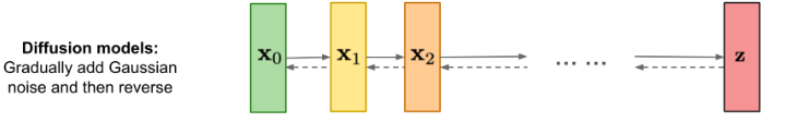
Figure 1 From CVPR 2022 Tutorial on Diffusion Models
A high level view of Diffusion Models is shown in Figure 1. A fully trained model generates images by taking a Latent Variable consisting of random noise data ${\bf z}$ to the right of the figure, and gradually ‘de-noises’ it in multiple stages as shown by the dotted arrows moving from right to left (typically 1000 stages in large networks such as DALL-E-2). This is done by feeding the output of stage $t$ to stage $t-1$, until we get to the final stage resulting in the image ${\bf x_0}$. This is illustrated in Figure 2, with the middle row illustrating the de-noising process starting from random data in stage $T$, followed by partially re-constructed image at stage ${T\over 2}$ and the final image at stage $0$.
Diffusion Models are trained by running the process just described in the opposite direction, i.e., from left to right in Figure 1, as shown by the solid arrows. An image ${\bf x_0}$ from the training dataset is fed into stage 1 resulting in image ${\bf x_1}$. This stage as well as the following ones add small amounts of noise to the image, so it becomes progressively more and more blurry, until all that is left at state $T$ is pure noise (this is illustrated in the top row of Figure 2). Since we know precisely how much noise is being added in each stage, the DDPM algorithm works by training a Neural Network to predict the added noise level given the noisy image data as the input into the model. This optimization problem is posed as that of minimizing a convex regression loss, which is a much simpler problem to solve as compared to the minmax approach in GANs.
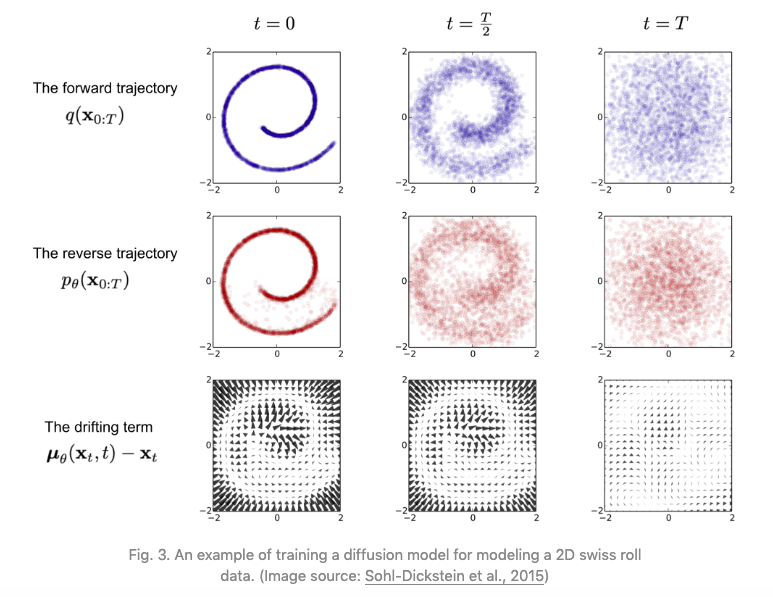
Figure 2 From Sohl-Dickstein
Latent Variables and the ELBO Bound
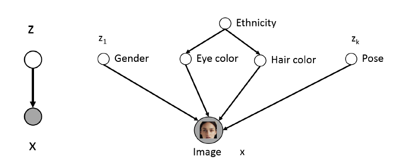
Figure 3 From Stanford CS236
Given a set of image samples $(X_1,…,X_N)$ we would like to estimate their Probability Density functions $q(X)$, so that we can sample from it and thereby generate new images. However, in general $q(X)$ is a very complex function, and a simpler problem is to define a Latent Variable $Z$ that encodes semantically useful information about $X$ and then estimate $q(X\vert Z)$ with the hope that this will be a simpler function to estimate. The idea behind Latent Variables is illustrated in Figure 3: The LHS of the figure shows how new images can be generated in a two step process: First sample a Latent Variable $Z$ assuming that we know its distribution $q(Z)$ and then sample from $q(X\vert Z)$ to generate a new image. The RHS of the figure gives some intuition behind the concept of Latent Variables, it shows how the contents of an image of a human face are controlled by variables such as gender, hair color etc, and if these variables are specified, then the face generation problem becomes simpler.
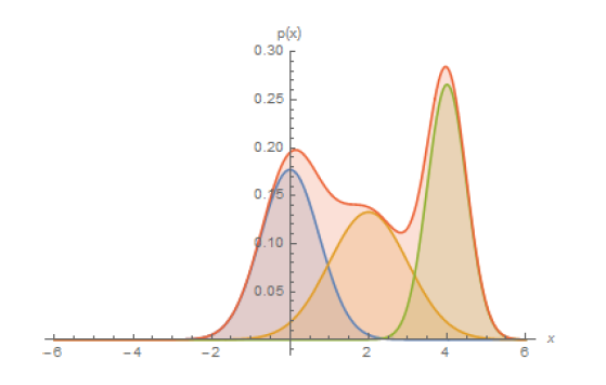
Figure 4 From Stanford CS236
For another perspective into the problem, consider Figure 4 which shows the data distribution $q(X)$ which in general can a very complicated function (as a stand-in for an image distribution). However note that by using the Law of Total Probabilities, $q(X)$ can also written as
\[q(X) = \int q(X,Z) dZ = \int q(X|Z) q(Z) dZ\]If $q(X\vert Z)$ is a simpler function that can be approximated by a Gaussian $p_\theta(X\vert Z) = p_\theta(\mu_\theta(Z),\sigma_\theta(Z))$ then
\[q(X) \approx \int p_\theta(\mu_\theta,\sigma_\theta) q(Z) dZ\]Thus a complex $q(X)$ can be built by using a number of of these Gaussians super-imposed togther and weighted by the distribution $q(Z)$ as shown in Figure 4. This is somewhat analogous to approximating a complex function by its Fourier Transform co-efficients which act as weights for simple sinusoidal functions.
We now show how to obtain the approximations $p_\theta(X\vert Z)$ by solving an optimization problem.
Evidence Lower Bound or ELBO is a useful technique from Bayesian Statistics, that has found use in Neural Network modeling in recent years. It works by converting the problem of estimating an unknown probability distribution into an optimization problem, which can then be solved using Neural Networks.
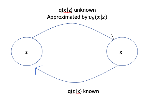
Figure 5
Consider the following problem: Given two random variables $X$ and $Z$, the conditional probabilities $q(Z\vert X)$ and $q(Z)$ are known, and we are asked to invert the conditional probability and thus compute $q(X\vert Z)$. For example $X$ may be an image so that $Z$ is the Latent Variable representation of the image. In this case the problem can be formulated as: We know how to get the latent representation from the image, but we don’t know how to convert a latent representation back into an image.
The most straightforward way of inverting the conditional probability is by means of Bayes Theorem, which states
\[q(X|Z) = {q(Z|X)q(x)\over{\sum_u q(Z|U)q(U)}}\]However this formula is very difficult to compute because the sum in the denominator is often intractable. In order to solve this problem using Neural Networks, we have to turn this into an optimization problem. This is done by means of a technique called ELBO (Evidence Lower Bound) also known as VLB (Variational Lower Bound), which works as follows: Lets assume that we can approximate $q(X\vert Z)$ by another (parametrized) distribution $p_\theta(X\vert Z)$. In order to find the best $p_\theta(X\vert Z)$, we can try to minimize the “distance” between $p_\theta(X\vert Z)$ and $q(X\vert Z)$. A measure of distance between probability distributions is the Kullback-Leibler Divergence or KL Divergence. The KL Divergence between probability distributions $f(X)$ and $g(X)$ is defined as:
\[D_{KL}(f(X), g(X)) = \sum f(X)\log{f(X)\over g(X)}\]Substituting $f(X) = q(X\vert Z)$ and $g(X) = p_\theta(X\vert Z)$, and making use of the Law of Conditional Probabilities, it can be shown that
\[D_{KL}(q(X|Z), p_\theta(X|Z)) = \log q(X) - \sum_Z q(Z|X)\log{ p_\theta(X,Z)\over q(Z|X)}\]Hence in order to minimize $D_{KL}(q(X\vert Z), p_\theta(X\vert Z))$, we have to maximize $\sum_Z q(Z\vert X)\log{ p_\theta(X,Z)\over q(Z\vert X)}$, or minimize $\sum_Z q(Z\vert X)\log{q(Z\vert X)\over p_\theta(X,Z)}$. We will refer to the latter quantity as the ELBO or VLB, i.e.,
\[ELBO = \sum_Z q(Z|X)\log{q(Z|X)\over p_\theta(X,Z)} \quad\quad\quad\quad (1)\]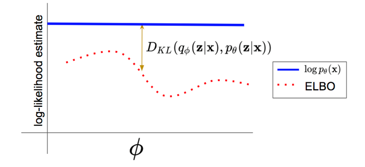
Figure 6 From Stanford CS236
Since by definition $D_{KL}(q(X\vert Z), p_\theta(X\vert Z)) \ge 0$, it follows that \(\log q(X) \ge ELBO\) i.e., the ELBO serves as an approximation to the true distribution $q(X)$, with the difference betwen the two being equal to the KL Divergence $D_{KL}(q(X\vert Z), p_\theta(X\vert Z))$ as illustrated in Figure 6.
Note: In Diffusion Approximations the distribution $q(Z\vert X)$ is known (as explained in the next section), however this is not the case in other Latent Variable models such as VAEs. In that case $q(Z\vert X)$ is also approximated by a parametrized distribution $q_\phi(Z\vert X)$, which is assumed to Gaussian as well. Thus building a VAE model requires a joint optimization of the parameters $(\theta,\phi)$.
Hence even though we don’t have access to the true distribution $q(X)$, we can approximate it using the ELBO, with the parameters $\theta$ (or $\theta,\phi$) being chosen so as to minimize the difference between the two.
The ELBO serves as a convenient optimization measure that can be used to train a Neural Network. To make the problem more tractable, it is also assumed that the unknown distribution $p_\theta$ belongs to the family of Gaussian distributions $N(\mu_\theta,\sigma_\theta)$, which reduces the problem to that of estimating its mean $\mu_\theta$ and variance $\sigma_\theta$. These quantities can be estimated by using a DLN with parameters $\theta$, with the ELBO serving as a Loss Function to optimize the network. This optimization procedure underlies Diffusion Models.
Forward Diffusion Process
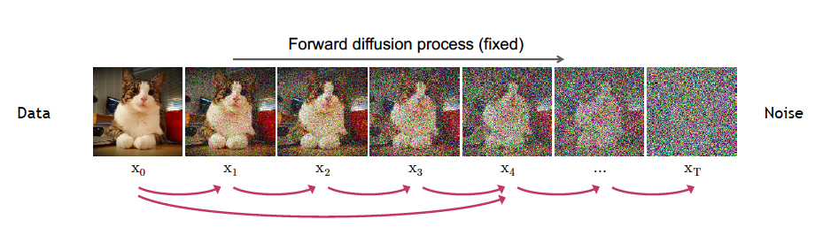
Figure 7 From CVPR 2022 Tutorial on Diffusion Models
Note: We will use the notation $N(X; \mu,\Sigma)$ for a mutivariate Gaussian (or Normal) Distribution $X$ with mean vector $\mu = (\mu_1,…,\mu_N)$ and covariance matrix $\Sigma$ (here is a a short introduction to multivariate Normal Distributions). For the special case when the covariance matrix is a diagonal with a common variance $\sigma^2$, this reduces to $N(X; \mu,\sigma^2 I)$ where $I$ is a $N\times N$ identity matrix.
Note: Given a Gaussian Distribution $N(X;\mu,\sigma^2 I)$, it is possible to generate a sample from it by using the Re-Parametrization Trick, which states that a sample $X$ can be expressed as
\[X = \mu + \sigma \epsilon\]where the random vector $\epsilon$ is distributed as per the Unit Gaussian Distribution $N(0,I)$.
The setup used in Diffusion Models is shown in Figure 7. We start with an image $X_0 = (x_{01},…,x_{0N})$, shown on the left. Note that even though $X_0$ is a 3D tensor, for this discussion we will flatten it out into a 1D vector. $X_0$ is distributed according to some unknown distribution $q(X_0)$ to which we don’t have access.
We gradually add small amounts of Gaussian Noise to $X_0$ in $T$ steps (typically T = 1000 in large models), such that at the $t^{th}$ step the resulting conditional distribution is given by the Gaussian
\[q(X_t|X_{t-1}) = N(X_t; \sqrt{1-\beta_t} X_{t-1}, \beta_t I)\]At this step the ‘signal’ $X_{t-1}$ in the image is suppressed by the factor $\sqrt{1-\beta_t}$, while an amount of noise $\beta_t$ is added to it, i.e., the image gets more and more blurry as $t$ increases. The sequence $\beta_i$ is chosen such that $\beta_1 < \beta_2 < … < \beta_T < 1$, i.e., the amount of noise being added increases monotonically, which is known as the Variance Schedule. This can be chosen to be linear, quadratic, cosine etc or even a learnt sequence.
By using the Re-parametrization Trick, we can sample $X_t$ from the distribution $q(X_t\vert X_{t-1})$
\[X_t = \sqrt{1-\beta_t}X_{t-1} + \sqrt{\beta_t}\epsilon_{t-1} \quad\quad\quad (2)\]where $\epsilon_{t-1}$ is sampled from the N Dimensional Gaussian distribution $N(0,I)$. From this equation it is clear that the sequence $X_t, 0\le t\le T$ forms a Markov Chain. This is also referred to as a Discrete Time Diffusion, and later we will see that if T is kept fixed while increasing the number of stages in the model, then there is a continuous time limit to Equation (2) as $T\rightarrow\infty$, resulting in $X_t$ converging to a continuous time Diffusion Process (in the index t) driven by a Weiner Process.
Since Equation (2) is a recursion in the $X_t$ sequence, we can show that the $X_t$ sample can also be expressed in terms of the starting image vector $X_0$ as follows:
\[X_t = \sqrt{\gamma_t} X_0 + \sqrt{1 - \gamma_t}\epsilon \quad\quad\quad (3)\]where $\epsilon$ is sampled from $N(0,I)$, and \(\gamma_t = \prod_{i=1}^t \alpha_i\) where $\alpha_t = 1 - \beta_t$. This equation allows us to get a sample of $X_t$ at the $t^{th}$ stage directly from original $X_0$ sample. This property is very useful when training the Neural Network since it allows us to optimize random terms of the Loss Function as we will see shortly.
Note that since the $\gamma_t$ sequence is a product of factors that are less than one, it follows that $\gamma_1 \ge\gamma_2\ge … \ge\gamma_T$. These sequences are chosen so that $\gamma_t\rightarrow 0$ as $t$ increases, and from equation (3) this implies that the distribution of $X_T$ approaches $N(0,I)$ which is also referred to as “white” noise. This is illustrated in Figure 8 which shows the distribution of a single pixel $x$, starting from the unknown distribution $q(x_0)$ on the left and ending up as the Standard Gaussian on the right.
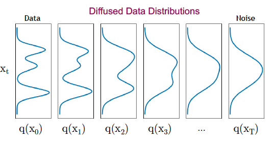
Figure 8 From CVPR 2022 Tutorial on Diffusion Models
Reverse Diffusion Process
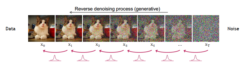
Figure 9 From CVPR 2022 Tutorial on Diffusion Models
In order to generate an image while starting from Gaussian noise, we need to reverse the process shown in Figure 7, i.e., we start with the white noise image $X_T$ sampled from Gaussian Noise $N(0,I)$ and then gradually “de-noise” this image as we move from right to left, as shown in Figure 9. In order to do so we need knowledge of the reverse distribution $q(X_{t-1}\vert X_t)$ which in general is an intractable problem. However we can try to approximate the reverse distribution with a parametrized distribution $p_\theta$ such that $p_\theta(X_{t-1}\vert X_t)\approx q(X_{t-1}\vert X_t)$. We will further assume that $p_\theta(X_{t-1}\vert X_t)$ has a Gaussian distribution given by
\[p_\theta(X_{t-1}|X_t) = N(X_{t-1};\mu_\theta(X_t,t),\sigma_\theta (X_t,t)I)\quad\quad\quad (4)\]where $\mu_\theta(X_t,t)$ and $\sigma_\theta(X_t,t)$ are complex and unknown functions parametrized by $\theta$. The Gaussian approximation to $q(X_{t-1}\vert X_t)$ works well for the case when the per stage added noise $\beta_t$ in the forward direction is sufficiently small.
If the distributions $p_\theta$ were known, then it is possible to recover the distribution of the original image as illustrated in Figure 10.
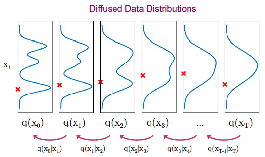
Figure 10 From CVPR 2022 Tutorial on Diffusion Models
Optimization Objective
Under the Gaussian asumption, the problem of finding the distributions $p_\theta(X_{t-1}\vert X_t)$ which best approximate $q(X_{t-1}\vert X_t)$ reduces to finding the parametrized functions $\mu_\theta$ and $\sigma_\theta$. In order to find the optimum set of parameters, we need to find a Loss Function whose minimization gives us these optimum parameters. Note that for a single stage this problem formulation falls within the purview of the ELBO technique. This can be extended across all the $T$ stages in the model as follows: Define the joint probabilities
\[p_\theta(X_{0:T}) = p(X_T)\prod_{t=1}^T p_\theta(X_{t-1}|X_t)\] \[q(X_{1:T}|X_0) = \prod_{t=1}^T q(X_t|X_{t-1})\]The ELBO optimization objective (see equation (1)) can be formulated as minimization of
\[L_{ELBO} = E_{q(X_{0:T})}{\log q(X_{1:T}|X_0) \over{p_\theta(X_{0:T})} }\]After some algebraic manipulations and making use of the Law of Conditional Probabilities, this expression can be re-written as
\[L_{ELBO} = E_q\left[{\log{q(X_T|X_0)\over{p_\theta}(X_T)}} + \sum_{t=2}^T \log{q(X_{t-1}|X_t,X_0)\over {p_\theta(X_{t-1}|X_t)}} - \log p_\theta(X_0|X_1)\right]\]which is the same as
\[L_{ELBO} = E_q\left[D_{KL}(q(X_T|X_0)||p_\theta(X_T) ) + \sum_{t=2}^T D_{KL}(q(X_{t-1}|X_t,X_0)||p_\theta(X_{t-1}|X_t) ) - \log p_\theta(X_0|X_1) \right]\]Defining
\[L_T = D_{KL}[q(X_T|X_0)||p_\theta(X_T) ]\] \[L_t = D_{KL}\left[q(X_t|X_{t+1},X_0)||p_\theta(X_t|X_{t+1})\right]\quad 1\le t\le T-1\] \[L_0 = - \log p_\theta(X_0|X_1)\]$L_{ELBO}$ can be written as
\[L_{ELBO} = L_T + L_{T-1} + ... +\ L_0\]In this expression the $L_T$ term can be ignored for optimization purposes since $q(X_T\vert X_0)$ being equal to $N(0,I)$ is not a function of $\theta$ and neither is $p_\theta(X_T)$. Even though $q(X_{t-1}\vert X_t)$ is an intractable distribution, it can be shown that $q(X_{t-1}\vert X_t,X_0)$ is actually a Gaussian distribution which makes the loss terms $L_t, 1\le t\le T-1$ computable. After some algebraic manipulations The parameters of this distribution can be computed as follows:
\[q(X_{t-1}|X_t,X_0) = N(X_{t-1}; {\tilde\mu}(X_t,X_0),{\tilde\beta_t} I) \quad\quad\quad (5)\]where
\[{\tilde\beta_t} = {1-\gamma_{t-1}\over{1-\gamma_t}}\beta_t\]and
\[{\tilde\mu}(X_t,X_0) = {\sqrt{\alpha_t}(1-\gamma_{t-1})\over{1-\gamma_t }}X_t + {\sqrt{\gamma_{t-1}}\beta_t\over{1-\gamma_t }}X_0 \quad\quad\quad (6)\]Note that we are trying to approximate $q(X_t\vert X_{t+1},X_0)$ by $p_\theta(X_t\vert X_{t+1})$ by minimizing \(L_t = D_{KL}[q(X_t\vert {X_{t+1},X_0})||p_\theta(X_t\vert X_{t+1})], 1\le t\le T-1\). Using the fact that $q(X_{t-1}\vert {X_t,X_0})$ has a Normal Distribution given by equation (5) and $p_\theta(X_t\vert X_{t+1})$ also has a Normal Distribution given by equation (4), and plugging them into the formula for $D_{KL}$ results in the following (see Wikipedia article on Multi-Variate Normal Distributions to see why), :
\[L_t = E \left[{1\over{2||\Sigma_\theta(X_t,t)||^2}} ||\tilde\mu_t(X_t,X_0) - \mu_\theta(X_t,t)||^2 \right]\quad 1\le t\le T-1 \quad\quad\quad (7)\]According to equation (7), we should design our Neural Network to learn $\mu_\theta$ while using $\tilde\mu_t$ as the ground truth.
However Ho et.al. discovered that the system performance improves if the Neural Network is trained to learn the Noise Level $\epsilon_t$ instead. This can be done by expressing $X_0$ in terms of $X_t$ and $\epsilon$ by using equation (3), so that
\[X_0 = {1\over\sqrt{\gamma_t}}(X_t - \sqrt{1-\gamma_t}\epsilon_t)\quad\quad\quad (8)\]Substituting $X_0$ into equation (6), results in
\[{\tilde\mu}(X_t,X_0) = {1\over\sqrt\alpha_t} \left[X_t - {\beta_t\over{\sqrt{1-\gamma_t}}}\epsilon_t\right]\]Note that in this equation $\epsilon_t$ is the noise that is added to the image $X_0$ during training in order to get $X_t$. We will get an estimate $\epsilon_\theta(X_t,t)$ of $\epsilon_t$ using a Neural Network, and plugging this back into equation (8) results in an estimate $\mu_\theta(X_t,t)$ given by
\[\mu_\theta(X_t,t) = {1\over\sqrt\alpha_t}\left[X_t - {\beta_t\over{\sqrt{1-\gamma_t}}}\epsilon_\theta(x_t,t)\right]\]Substituting these equations back into (7), we get
\[L_t = E \left[{1\over{2||\Sigma_\theta(X_t,t)||^2}} ||{1\over\sqrt\alpha_t}(X_t - {\beta_t\over{\sqrt{1-\gamma_t}}}\epsilon_t) - {1\over\sqrt\alpha_t}(X_t - {\beta_t\over{\sqrt{1-\gamma_t}}}{\epsilon_\theta}(X_t,t))||^2\right]\] \[= E\left[{\beta_t^2\over{2\alpha_t(1-\gamma_t) ||\Sigma_\theta(X_t,t)||^2}} || \epsilon_t - {\epsilon_\theta}(X_t,t)||^2 \right]\] \[= E \left[{\beta_t^2\over{2\alpha_t(1-\gamma_t) ||\Sigma_\theta(X_t,t)||^2}} ||\epsilon_t - \epsilon_\theta(\sqrt\gamma_t X_0 + \sqrt{1-\gamma_t}\epsilon_t,t)||^2 \right]\]Ho. et.al. also discovered that training the diffusion model is easier if the weighting term is ignored, so that the optimization problem becomes
\[L_t^{simple} = E\left[||\epsilon_t - \epsilon_\theta(\sqrt\gamma_t X_0 + \sqrt{1-\gamma_t}\epsilon_t,t)||^2 \right]\]The DDPM Algorithm
We collect all the results from the previous sections and put them together in the DDPM algorithm described below.
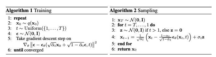
Figure 11 From Ho, Jain, Abbeel
The pseudocode for the training procedure is shown on the left in Figure 11, and proceeds as follows:
- An image is sampled from the training dataset, with (unknown) distribution $q(X_0)$
- A single step index $t$ of the forward diffusion process is sampled from the set ${1,…,T}$, using an Uniform Distribution
- A random noise vector $\epsilon$ is sampled from the Gaussian Distribution $N(0,I)$
- The noisy image $X_t$ is sampled at the $t^{th}$ step, given by $X_t = \sqrt\gamma_t X_0 + \sqrt{1-\gamma_t}\epsilon$. This is then fed into the Deep Learning model to generate an estimate of the noise that was added to $X_0$ in order to obtain $X_t$, given by $\epsilon_\theta(\sqrt\gamma_t X_0 + \sqrt{1-\gamma_t}\epsilon,t)$.
- The difference between the actual noise sample $\epsilon$ and its estimate $\epsilon_\theta$ is used to generate a gradient descent step.
Once we have a trained model, we can use it to generate new images by using the procedure outlined in Algorithm 2. At the first step we start with a Gaussian noise sample $X_T$, and then gradually de-noise it in steps $X_{T-1}, X_{T-2},…,X_1$ until we get to the final image $X_0$. The de-noising is carried out by sampling from the Gaussian Distribution $N(\mu_\theta(X_t,t),\beta_t I)$, so that
\[X_{t-1} = \mu_\theta(X_t,t) + \sqrt{\beta_t} \epsilon\]$\mu_\theta(X_t,t)$ is computed by running the model to estimate $\epsilon_\theta$ and then using the following equation to get $\mu_\theta$
\[\mu_\theta(X_t,t) = {1\over\sqrt\alpha_t}\left[X_t - {\beta_t\over{\sqrt{1-\gamma_t}}}\epsilon_\theta(X_t,t)\right]\]Note that images are generated in a probabilistic manner starting from the initial Gaussian noise $X_T$, so that the same noise sample can generate different images on successive runs (which accounts for the P in DDPM).
The Neural Network
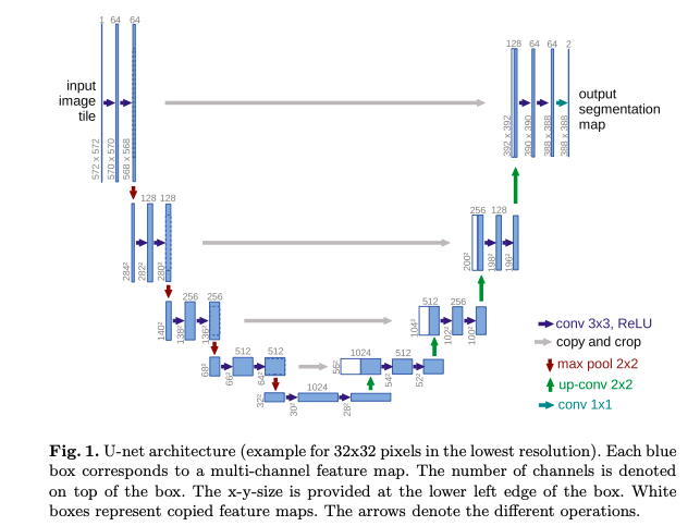
Figure 12 From Ronneberger et.al.
A Neural Network which would be appropriate for this application would be one that takes an input image and converts it another image of the same dimensions at the output. The class of networks that do this are called Auto-Encoders, and the one that was chosen for the job is called U-net (Ronneberger et.al, see Figure 12). A short description of this network follows:
- The Encoder part of the network consists of a series of cascaded ConvNets, with a combination of $3\times 3$ filtering and progressive downsampling (using max-pooling) during which the size of the image is steadily reduced. This is followed by upsampling in the Decoder part of the network.
- U-net uses Residual Connections that connect the Encoder and Decoder sections. This was inspired by ResNet and results in improved performance.
- Note that this network is shared across all the T stages in the Diffusion Model. Just as in Transformers, information about the stage number is encoded using a Position Embedding (see Figure 13).
- Though not shown in the figure, the network also includes Self Attention modules that were added in between the ConvNet layers, along with Group Normalization.
Another implementation decision is the schedule to be used for adding noise to the Diffusion stages using the sequence $\beta_t, 1\le t\le T$. We progressively increase the amount of noise added as $t$ increases so that $\beta_1 < \beta_2 < … < \beta_T$. In the original paper the authors employed a linear schedule with $\beta_1 = 10^{-4}$ to $\beta_T = 0.02$. Later it was discovered that a cosine schedule works better (see Dhariwal and Nichol).
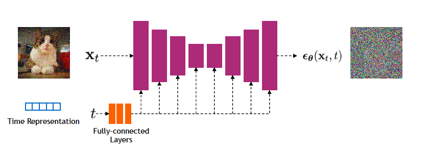
Figure 13 From CVPR 2022 Tutorial on Diffusion Models
Speeding Up Diffusion Models: The DDIM Algorithm
One of the issues with the DDPM algorithm is that the inference (or test) step takes too long to generate image, due to the 1000 or so times that the model has to be run in order to generate a single image. For example it takes about 20 hours to to sample 50k images of size $32\times 32$ from a DDPM on a Nvidia 2080 Ti GPU. The large number of steps are required, since the backward process is trying to approximate the forward Gaussian diffusion process, and the approximation improves if the smaller amounts of noise are introduced at every step.
Song, Meng,and Ermon came up with an ingenous way to speed up these models. They made the observation that DDPM did not really make use of the Markovian nature of the forward diffusion process anywhere in the algorithm. So perhaps if the forward diffusion were to be replaced by a non-Markovian process, then the number of steps in the backward process could be reduced, thus speeding up the algorithm. This resulted in an algorithm they called Denoising Diffusion Implicit Model or DDIM, which indeed works much faster.
Song et.al. used a slightly different parametrization of the forward diffusion process, which is described next. The forward recursion in DDPM is written as
\[q(X_t|X_{t-1}) = N(\sqrt{\alpha_t\over\alpha_{t-1}}X_{t-1}, (1-{\alpha_t\over\alpha_{t-1}})\epsilon),\quad \epsilon\in N(0,I)\]which results in
\[X_t = \sqrt{\alpha_t}X_0 + \sqrt{1-\alpha_t}\epsilon\]so that the convergence of $X_T$ to White Gaussian happens if $\alpha_T\rightarrow 0$. The DDPM objective is given by
\[L_\gamma(\epsilon_\theta) = \sum_{t=1}^T \gamma_t E_q\left[||\epsilon_\theta^{(t)}(\sqrt{\alpha_t}X_0 + \sqrt{1-\alpha_t}\epsilon_t) - \epsilon_t||^2 \right]\]Song et.al. made the following observations:
- Since the generative model approximates the reverse of the inference process, we need to re-think the inference process to reduce the number of iterations required by the generative model.
- The DDPM objective $L_\gamma$ only depends on the marginals $q(X_t\vert X_0)$ but not directly on the joint $q(X_{1:T}\vert X_0)$. Since there are many inference distributions with the same marginals, perhaps a non-Markovian inference distribution will lead to a more efficient generative processes.
Song et.al. came up up with a non Markovian inference process that has the same marginal, and further demonstrated that this process has the same surrogate objective function as DDPM. This meant that the trained DDPM models could be re-used by making use of the DDIM algorithm for generation only, with a faster execution time.
Consider the family Q of inference distributions indexed by a real vector $\sigma \in R^T_{\ge 0}$:
\[q_\sigma(X_{1:T}|X_0) = q_\sigma(X_T|X_0)\prod_{t=2}^T q_\sigma(X_{t-1}|X_t, X_0)\]where $q_\sigma(X_t\vert X_0) = N(\sqrt{\alpha_T}X_0, (1-\alpha_T)\epsilon)$ and for all $t>1$
\[q_\sigma(X_{t-1}|X_t,X_0) = N(\sqrt{\alpha_{t-1}}X_0 + \sqrt{1-\alpha_{t-1}-{\sigma_t}^2}. {X_t - \sqrt{\alpha_t}X_0\over{\sqrt{1-\alpha_t}}}, {\sigma_t}^2 \epsilon) \quad\quad\quad (9)\]Using this formula, it can be shown that $q_\sigma(X_t\vert X_0) = N(\sqrt{\alpha_t}X_0, (1-\alpha_t)\epsilon), \forall t$ so the marginals between this inference process and the DDPM forward process match. The forward process itself can be computed by using the formula:
\[q_\sigma(X_t|X_{t-1},X_0) = {q_\sigma(X_{t-1}|X_t,X_0)q_\sigma(X_t|X_0)\over{q_\sigma(X_{t-1}|X_0)}}\]This is clearly a Gaussian process, however note that $q_\sigma(X_t\vert X_{t-1},X_0)$ is not a Markov process, since $X_t$ depends on $X_0$ in addition to $X_{t-1}$.
Let $p_\theta(X_{0:T})$ be the Generative process, where ${p_\theta}^{(t)}(X_{t-1}\vert X_t)$ is approximated using $q_\sigma(X_{t-1}\vert X_t,X_0)$. This is done in a 2-step process:
- Given $X_t$, use it to predict $X_0$ (referred to as ${\hat X_0)}$) by using the Neural Network model and the equation
- Given $X_t$ and ${\hat X_0}$, use $q_\sigma(X_{t-1}\vert X_t,X_0)$ to sample $X_{t-1}$ so that
Note that changing the parameter $\sigma$ results in different generative processes, while using the same DDPM based training process. Some special choices of $\sigma$ are the following:
- When
\(\sigma_t = \sqrt{ {1-\alpha_{t-1}\over{1-\alpha_t}} }\sqrt{ 1-{\alpha_t\over\alpha_{t-1}} }, \quad\forall t\) then the forward process becomes Markovian and the generative process becomes DDPM.
- When $\sigma_t = 0,\forall t$ , the forward process becomes deterministic given $X_{t-1}$ and $X_0$, except for $t=1$. The generative process is now called an implicit probabilistric model where samples are generated from the latent variable $X_T$ with a fixed procedure.
DDIM Accelerated Sampling Process
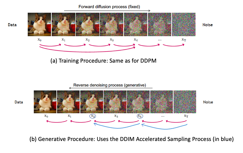
Figure 14 From CVPR 2022 Tutorial on Diffusion Models
Song et.al. made use of the fact that the $X_t$ sequence need not be Markov and proposed the following Accelerated Sampling Process:, which is illustrated in Figure 14:
As Part (a) of the figure shows, we can still use the same training procedure as DDPM, since DDPM and DDIM share the same Loss Function.
The Generative Procedure however is different. As shown in Part (b) of the figure, instead of doing Generation on all T steps, DDIM chooses an increasing sub-sequence $\tau=[\tau_1,\tau_2,…,\tau_S]$ of the forward sequence $[1,…,T]$ of length S with $\tau_S = T$, and then does generation only over this sub-sequence (shown using the blue arrows in the figure, assuming that $2$ and $4$ belong to $\tau$. Clearly $X(\tau_1),…,X(\tau_S)$ don’t form a Markov Chain, but as long as the forward process $q_\sigma(X_{\tau_{i-1}}\vert X_{\tau_i},X_0)$ satisfies equation (9), i.e.,
\[q_\sigma(X_{\tau_{i-1}}|X_{\tau_i},X_0) = N(\sqrt{\alpha_{\tau_{i-1}}}X_0 + \sqrt{1-\alpha_{\tau_{i-1}}-{\sigma_{\tau_i}}^2}. {X_{\tau_i} - \sqrt{\alpha_{\tau_i}}X_0\over{\sqrt{1-\alpha_{\tau_i}}}}, {\sigma_{\tau_i}}^2 \epsilon)\]where the coefficients $\sigma$ are chosen so that
\[q_{\sigma,\tau}(X_{\tau_i}|X_0) = N\left[\sqrt{\alpha_{\tau_i}}X_0, (1 - \alpha_{\tau_i})\epsilon\right],\quad \forall i\in S\]The reverse process conditionals are given by
\[{p_\theta}^{(\tau_i)}({X_{\tau_{i-1}}|X_{\tau_i}}) = q_{\sigma,\tau}(X_{\tau_{i-1}}|X_{\tau_i},{\hat X_0})\]where
\[{\hat X_0} = {( X_{\tau_i} - \sqrt{1-\alpha_{\tau_i}}.{\epsilon_\theta}^{(\tau_i)}(X_{\tau_i}))\over{\sqrt{\alpha_{\tau_i}}}}\]The generative process now samples latent variables according to the reversed $\tau$, which is referred to as the sampling trajectory. If the length of the sampling trajectory $S$ is much smaller than $T$, then it leads to significant speed-ups in the computational efficiency. DDIM is able to produce samples with quality comparable to 1000 step models within 20 to 100 steps. Indeed Song et.al. showed that only 20 steps are already very similar to the ones generated with 1000 steps in terms of high level features, with only minor diffferences in details.
The Latent Diffusion Model (LDM)
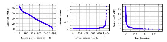
Figure 15 From Ho, Jain, Abbeel
Ho et.al. made the following interesting observation in their DDPM paper: During the inference process, we can regard the process of generating progressively better images from $X_T$ to $X_0$ in the following two ways:
- We can measure the image Distortion at stage $t$, which is defined as
\({ \sqrt{ \left\vert X_0 - {\hat X_0}\right\vert^2}\over D }\), where ${\hat X_0}$ is the prediction that the system makes for $X_0$, given $X_t$. This will give us some idea of how the predicted image quality changes with $t$ as the inference proceeds. This is graphed in the LHS of Figure 15.
- We can regard the process of predicting $X_0$ as an Information Theoretic problem, with each $X_t$ providing information on how to generate $X_0$. As we incorporate more and more information into ${\hat X_0}$, it gradually converges to $X_0$. This added information is referred to as the Rate, and is graphed in the middle graph of Figure gen16.
The curve on the left shows that there is an initial very steep decrease in the Distortion for small values of $T - t$, followed by a linear decrease. The Rate curve on the other hand shows that little information is passed on to ${\hat X_0}$, until the very end of the reverse process, at which point there is a very steep increase in Rate.
By definition, Distortion is a measure of difference between the pixel content of $X_0$ and ${\hat X_0}$. For example if two images have the same shapes, but are textured differently, then they will have a large distortion (another way of putting this is that Distortion measures the difference between the high frequency content in the two images). Rate on the other hand is a measure of semantic content, i.e., the specific objects in the image and how they relate to each other. These curves show that the initial stages in the reconstruction process have information about the texture or finer details of the image, while the later stages have information about the semantic content of the image.
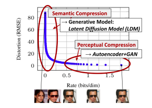
Figure 16 From Rombach, Emmer et.al.
This is further illustrated in Figure 16 that plots Distortion vs Rate, which shows that the inference process can be divided into two parts: Part 1 is referred to as Semantic Compression and leads to steep decrease in Distortion, while Part 2 is referred to as Perceptual Compression, and leads to increase in the semantic content of the re-constructed image. Rombach, Ommer et.al. made the observation that Diffusion Models excel at generating the semantic content of an image, but spend a lot of their processing in the generation of the perceptual content. This leads to the idea of breaking up the image generation process into two parts resulting in a model called the Latent Diffusion Model or LDM (see Figure 17).
-
Part 1 of the model (in red) consists of an autoencoder whose Encoder $E$ converts the original image $X$ into a lower dimensional image $Z$ in the Latent Space that is perceptually equivalent to the image space, but a significantly reduced computational complexity (since the high frequency, imperceptible details are abstracted away). This autoencoder is trained by a combination of perceptual loss and patch based adversarial objective (see Esser, Rombach, Ommer).
-
A Diffusion Model is then run on this modified image (in green). The reconstructed image $Z$ is fed into the Decoder of the Auto Encoder to get the final image ${\hat X_0}$. Since the Diffusion Model operates on a much lower dimensional space, they are much more computationally efficient. Also it can focus on important, semantic bits of data rather than the imperceptible high frequency content.
Given an input image $X\in R^{H\times W\times C}$ in RGB space, the Encoder encodes $X$ into the latent representation $Z\in R^{h\times w\times c}$, where $f={H\over h} = {W\over w}$ is the downsampling factor. Rombach, Ommer et.al. discovered that $f=4$ to $16$ strikes a good balance between efficiency and perceptually faithful results.
The LDM Model has been shown to produce images that are comparable in quality to DDPM/DDIM models, while using much less computational resources. As a result they form the core of the Solid Diffusion model that was released recently to the general public (see Solid Diffusion).
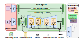
Figure 17 From Rombach, Emmer et.al.
Conditional Diffusion Models
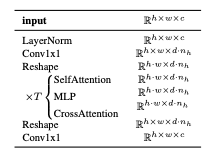
Figure 18 From Rombach, Emmer et.al.
The LDM model in Figure 17 also incorporates support for conditional image generatiom, where the condition could be a piece of text, images etc. Considering the case when text is used as the input, then the system works as follows:
-
As shown in the box on the right, the tokenized input $y$ is first passed through a network $\tau_\theta$ that converts it into a sequence $\zeta^{M\times d_{\tau}}$, where $M$ is the length of the sequence and $d_{\tau}$ is the size of the individual vectors. This conversion is done by means of an unmasked Transformer that is implemented using $N$ Transformer blocks consisting of global self-attention, layer-normalization and position-wise MLP layers.
-
$\zeta$ is mapped on to each stage of the de-noising section of the Diffusion Model using a cross-attention mechanism as shown in Figure 17. In order to do so, the Self Attention modules in the ablated UNet model (see Dhariwal and Nichol for a description) are replaced by a full Transformer consisting of T blocks of with alternating layers of self-attention, position-wise MLP and cross-attention. The exact structure is shown in Figure 18, with the shapes of the various layers involved.
The Cross Attention is implemented by using the flattened “image” tensor of shape $h.w\times d.n_h$ to generate the Query, and using the text tensor of shape $M\times d_\tau$ to generate the Key and Value.