Energy Based Models Part 2: Hopfield Networks and Boltzmann Machines
Contents
- Introduction
- Hopfield Networks: Engineering the Energy Landscape
- Thermodynamics of the Hopfield Network
- Modern Hopfield Networks
- From Hopfield Networks to Boltzmann Machines
- Training the Boltzmann Machine
- Restricted Boltzmann Machines
- Thermodynamics of the RBM
Introduction
This post is a continuation of Energy Based Models Part 1: Ising and Spin Glass Models.
Spin glasses by themselves haven’t become commercially important as materials, but the models that were built to explain their behavior had an unexpected side effect. They inspired the neural network models that were proposed in 1980s, initially by John Hopfield at Caltech, and later by Geoffrey Hinton and his collaborators. Hopfield regarded his network as a type of spin glass, more precisely as a modified SK model, and showed that the system can be made to function as an associative memory. Hopfield’s great insight was the realization the interaction between spins in his model could be chosen in a manner such that it resulted in as many phases as there are memories to the stored, and moreover the equilibrium spin configuration in each phase corresponds with one of the stored memories. Hence if the system is initialized in a state that is near a stored memory, then it gradually settles into an equilibrium configuration that corresponds to that memory.
Hinton and Sejnowski were inspired by Hopfield’s work, but they asked a different question. Instead of trying to remember the exact bit patterns, which is what the Hopfield network does, what if a network could be used to generate samples from the (unknown) probability distribution that the training data was drawn from. This is a very important problem in practice, for example consider the following: We have a bunch of N dimensional training data samples $(x_1,…,x_N)$ drawn from some unknown probability distribution $q(x_1,…,x_N)$. For example a sample could be an N pixel image, with each pixel assuming either black or white values. If the network can be trained to learn this probability distribution, then it can used it to generate new samples and thus the network would become a generator of new images similar to those in the training dataset. This was the very beginning of the field of generative AI which has assumed such gigantic importance in the present day, with LLMs being the prime example. Hinton and Sejnowski named their network the Boltzmann machine, the reason being that the equilibrium Boltzmann distribution $p$ of the spins in their network served as an approximation to the unknown probability distribution $q$. How were they able to accomplish this? They did it introducing the idea of learning the inter-node interactions (or weights) from the training data such that the ‘distance’ between the distributions $p$ and $q$ is minimized. The neural networks that that we use today are a direct descendant of these early models and use similar principles.
Hopfield Networks: Engineering the Energy Landscape of a Spin Glass System
The physicist John Hopfield was at Princeton during the 1970s, and he was instrumental in luring away Phil Anderson from Bell Labs to Princeton during that time. Anderson acquainted Hopfield with his work in spin glasses (see the Edwards-Anderson model in Part 1), and Hopfield began thinking about how these results could be applied to model biological systems. He hit upon the idea of creating an energy landscape with multiple valleys, and wondered if the equilibrium spin configuration in each valley (at T = 0) could be used as an associative memory. Subsequently he succeeded in creating a spin glass inspired model which indeed could do so, as explained next.
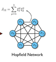
Figure 1: A Hopfield Network
Hopfield started with a SK type spin glass model with full connectivity, as shown above, with the symmetric interaction between nodes $i$ and $j$ given by $J_{ij}$. Assume that the spin at each node, $\sigma_i, i = 1,2,…N$ in the network can assume values of +1 or -1, and denote the state $X$ of the network as $\Sigma = (\sigma_1,…,\sigma_N)$. Furthermore assume that the state of the network evolves according to the equation
\[\sigma_i(t+\Delta t) = sign(\sum_{j\ne i}^N J_{ij} \sigma_j(t))\]where $\sum_{j\ne i}^N J_{ij} \sigma_j(t)$ is the local field acting on node $i$ and each node randomly and asynchronously evaluates whether it is above or below its threshold, and adjusts its value accordingly. This rule can be derived from the Glauber dynamics that we encountered in Part 1, when specialized to the case $T=0$, and is known as Gibbs sampling. We will have more to say about this in the following sections.
Given the update rule, this model has energy function given by
\[E = -{1\over 2}\sum_{i=1}^N\sum_{j=1}^N J_{ij}\sigma_i\sigma_j\]which is the same as that used for spin glass systems. If we are to use this system as a memory, there should be a way to choose the interactions $J_{ij}$ so that the energy minima correspond to bit patterns that we want to store. In order to achieve this, Hopfield hit upon the novel idea of engineering the energy landscape by choosing the interactions to be a function of the bit patterns to be stored in the associative memory.
Assume that we wish the network to store the vector states $\Xi^s, s=1,…,p$ so that the $\mu^{th}$ excitation pattern can be written as $\Xi^\mu=(\xi^\mu_1,…,\xi^\mu_N)$. In order to store these states, Hopfield proposed that the interactions $J_{ij}$ be chosen according to the Hebb rule
\[J_{ij} = {1\over N}\sum_{\mu=1}^p \xi^\mu_i \xi^\mu_j\ \ \ with\ \ \ J_{ii} = 0\]Clearly the interaction strengths $J_{ij}$’s can assume both positive and negative values, so the system qualifies as a spin glass, but not of the Sherrington-Kirkpatrick kind, since the $J_{ij}$’s are not Normally distributed. After substituting for $J_{ij}$, $E$ can be written as
\[E = -{1\over 2N}\sum_{\mu=1}^p(\sum_{i=1}^N \sigma_i\xi^\mu_i)^2\]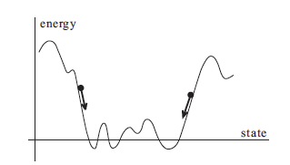
Figure 2: Energy landscape and time evolution
The spin updates cause a monotonically decreasing value of the energy (see above figure), since if there is a change $\Delta\sigma_i$ in the value of the $i^{th}$ spin, then
\[\Delta E = -{1\over 2}\Delta\sigma_i \sum_{j} J_{ij}\sigma_j\]and the signs for $\Delta\sigma_i$ and $\sum_j J_{ij}\sigma_j$ coincide. These state changes with decreasing energy will continue until a stable point such as one of the stored memories $\xi^\mu$ is reached. The above figure shows this situation where the network reaches a minimum of energy closest to the initial condition and stops there. Note that there is no thermal disorder in the model, so the system settles at the bottom of the nearest valley. But does it converge to one of the stored states? Using simulations Hopfield showed that in most cases it does. However the memory retrieval reliability goes down as more and more states are stored, and about $0.15N$ states can be simultaneously remembered before the error in recall is severe.
How did Hopfield arrive at his formula for the interactions $J_{ij}$? In the 1940s artificial neural networks pioneer Donald Hebb proposed that the strength of the synaptic connection between two biological neurons increases every time the two neurons fire together. The equation for $J_{ij}$ captures this by making it proportional to the number of locations in which the $\xi^\mu_i$ and $\xi^\mu_j$ coincide for $\mu=1,…,p$. In order to get some intuition for this, consider the example in which a network with $N=3$ nodes is being used to store the following three vectors:
\[\Xi^a = (\xi^a_1,\xi^a_2,\xi^a_3)\] \[\Xi^b = (\xi^b_1,\xi^b_2,\xi^b_3)\] \[\Xi^c = (\xi^c_1,\xi^c_2,\xi^c_3)\]This can also be regarded as a system in which the vector $\Xi_1=(\xi^a_1,\xi^b_1,\xi^c_1)$ is associated with node 1, the vector $\Xi_2=(\xi^a_2,\xi^b_2,\xi^c_2)$ is associated with node 2 and the vector $\Xi_3=(\xi^a_3,\xi^b_3,\xi^c_3)$ is associated with node 3. The strength of connection between nodes 1 and 2 is proportional to the number of locations in $\Xi_1$ and $\Xi_2$ which are equal. If $\Xi_1$ and $\Xi_2$ are closer to each other then this causes the value of $J_{12}$ increase, and this in turn causes the spin values $\sigma_1$ and $\sigma_2$ at the two nodes tend to draw closer to each other, and vice-versa. Hence, assuming $\sigma_1=\xi^a_1$ and $\xi^a_1 = \xi^a_2$, then $\sigma_2$ will tend to be equal to $\sigma_1$.
Assuming that the network is at one of the stored states $\Xi^\mu$, what are the chances that it continue to stay in this state after updates? A single step of the state evolution leads to the following spin value $\sigma_i$ at node $i$:
\[\sigma_i = sign(\sum_{j=1}^N J_{ij}\xi^\mu_j) = sign{1\over N} (\sum_{j=1}^N\sum_{\nu=1}^p \xi^\nu_i \xi^\nu_j \xi^\mu_j)\]Splitting this sum to the case $\nu=\mu$ and the rest, it follows that
\[\sigma_i = sign(\xi^\mu_i + {1\over N} \sum_{j=1}^N \xi^\mu_j\sum_{\nu\ne\mu} \xi^\nu_i \xi^\nu_j)\]The second term is called the crosstalk term (since it is influence of all the other memories on $\Xi^\mu$), and if its absolute value is less than $1$ for all $i$, then it follows that $\sigma_i = \xi^\mu_i$, i.e., the pattern $\Xi^\mu$ is a fixed point for the network.
It is possible to obtain a rough estimate for the capacity of the Hopfield network by analyzing the crosstalk term, and this is done next. In general the crosstalk increases as the number $p$ of stored patterns increases, and we want to find an upper bound for $p$, such that the crosstalk term remains small enough with high probability. Multiply the crosstalk term by $-\xi^\mu_i$ to obtain
\[C_i^\mu = -\xi^\mu_i {1\over N} \sum_{j=1}^N \xi^\mu_j\sum_{\nu\ne\mu} \xi^\nu_i \xi^\nu_j\]Note that if $C_i^\mu$ is negative then the crosstalk term has the same sign as $\xi^\mu_i$, and thus it will not cause a change in its sign. On the other hand if $C_i^\mu$ is positive and greater than 1, then the sign of $\sigma_i$ will change, which will lead to an error in the memory retrieval.
We will estimate the probability $P(C_i^\mu >1)$. Assume that $\xi_i^\nu, 1\le i\le N, 1\le\nu\le p$ are purely random with equal probabilities of being $1$ and $-1$. Thus $C^\mu_i$ is the sum of (roughly) $Np$ independent and identically distributed random variables, say $y_m, 1\le m\le Np$ with equal probabilities of being $1$ and $-1$. Since $E(y_m)=0$ and $Var(y_m) = 1$ for all $m$, it follows from the central limit theorem that $C_i^\mu$ has approximately a Normal distribution with $N(0,s^2)$ with mean $0$ and variance $s^2 = {p\over N}$. Therefore if we store $p$ patterns in a Hopfield network with $N$ nodes, then the probability of error is given by
\[P_{error} = P(C^\mu_i > 1) \approx {1\over 2}(1-erf(\sqrt{N\over{2p}}))\ \ \ with\ \ \ erf(x) = {1\over\sqrt{\pi}}\int_0^x e^{-s^2} ds\]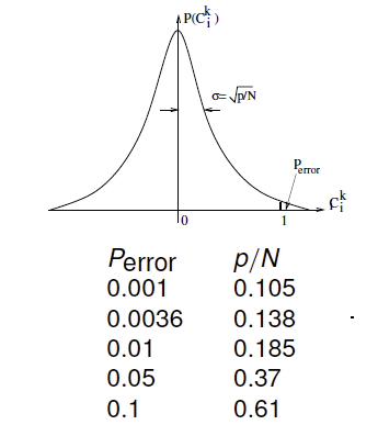
Figure 3: Error probability in a Hopfield network
The table above shows the error for some values of ${p\over N}$. We can see that error is reasonably low until ${p\over N}=0.138$, and increases sharply after that. This estimate has been borne out by a more thorough analysis of Hopfield networks using the tools from spin glass theory.
The argument presented in this section for memory recall was of the fixed point type, i.e., if the system was already in one of the memory states, then it will tend to stay there (provided $p<0.138N$). But under normal operations the system will be initialized to some arbitrary state, and if so, will it still converge to one of the memory vectors? It turns out that there are energy minima in the Hopfield network that don’t correspond to any of the stored patterns, and there is a chance that the system will end up at one of those. What is the nature of these minima, and what can be done to avoid getting stuck in them? In order to answer these questions we have to introduce thermal disorder, i.e., temperature, into the system, which allows the use of the tools from statistical mechanics that we learnt in Part 1.
Thermodynamics of the Hopfield Network
The classic reference for the material in this section is the paper by Amit, Gutfreund, Sompolinsky. A more accessible description can also be found in Nishimori’s book.
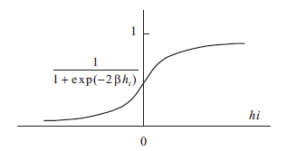
Figure 4: The probability that node $i$ becomes excited
We make the following change to the state transition equations in order to take thermal dynamics into account: Denote the field at node $i$ at time $t$ as
\[h_i(t) = \sum_j J_{ij}\sigma_j(t)\]and assume that $\sigma_i(t+\Delta t)$ becomes 1 with probability $1\over{1+e^{-2\beta h_i(t)}}$ and -1 with probability ${e^{-2\beta h_i(t)}\over{1+e^{-2\beta h_i(t)}}}$, where $\beta = {1\over T}$ is the inverse temperature (see above figure). Note that this stochastic dynamics reduces to earlier state transition equation in the limit $\beta\rightarrow\infty$ so that the original Hopfield Network corresponds to the case $T=0$, since $\sigma_i(t+\Delta t) = 1$ if $h_i(t) > 0$ and is $\sigma_i(t+\Delta t) = -1$ otherwise. On the other hand the network becomes completely random if $T=\infty$. From our knowledge of statistical mechanics, we know that if the system is allowed to evolve then ultimately it will settle down to a set of states whose probabilities are distributed according to the Boltzmann distribution.
Lets assume we are trying to store the $p$ patterns $\Xi^\mu = (\xi^\mu_1,…,\xi^\mu_N), \mu = 1,…p$. For this case, the partition function $Z$ for the Hopfield network is given by
\[Z = \sum_{[\sigma]} \exp[{\beta\over{2N}}\sum_{\mu=1}^p ( \sum_{i=1}^N \sigma_i\xi^{\mu_i} )^2]\]where the first sum is over all possible spin patterns $[\sigma]$, and the effect of the diagonal terms $J_{ii} = 0$ has been ignored since there are much fewer of these terms in the sum. The next step is to apply the Hubbard-Stratonovich transformation to the term in the exponent, which results in
\[Z = \sum_{[\sigma]} \int\prod_{\mu=1}^p dm^{\mu}\ \exp[-{1\over{2}}N\beta \sum_{\mu}(m^{\mu})^2 + \beta\sum_{\mu} m^{\mu}\sum_{i} \sigma_i\xi^{\mu}_i ]\]This transformation results in the introduction of the integration variables $m^{\mu}, i=1,…,p$. Using the notation $M = (m^1,…,m^p)$ and $\Xi_i = (\xi^1_i,…,\xi^p_i)$ (note that this is just the set of memory bits associated with node i), if we sum over all possible values of the spin patterns $[\sigma]$, then this results in
\[Z = \int\prod_{\mu=1}^p dm^{\mu}\ \exp[-{1\over{2}}N\beta M.M + \sum_{i=1}^N \log(2\cosh\beta M.\Xi_i) ]\]Recall that the free energy density $f$ is given by
\[f = -{1\over{\beta N}} \log Z\]If $N$ is very large the integral over $m^\mu$ is dominated by its saddle point value, so that $f$ can be approximated as
\[f = {1\over 2} M_{sp}.M_{sp} - {1\over{\beta N}} \sum_i \log(2\cosh\beta M_{sp}.\Xi_i)\]The order parameter vector vector $M_{sp}$ is determined by the saddle-point equation ${\partial f\over{\partial m^{\mu}}} = 0$ which results in
\[m^\mu_{sp} = {1\over N} \sum_{i=1}^N \xi_i^\mu \tanh(\beta M_{sp}.\Xi_i),\ \ \ \mu=1,...,p\]Both $f$ and $M$ depend on the contents of the memory values $\xi_i^\mu, \mu = 1,…,p, i = 1,…,N$, but in the limit as $N\rightarrow\infty$, we can invoke the averaging principle whuch results in the free energy density ${\overline f}$ given by
\[{\overline f} = {1\over{2}} M_{sp}.M_{sp} - {1\over\beta} <\log(2\cosh\beta M_{sp}.\Xi)>\]and
\[m^\mu_{sp} = <\xi^\mu\tanh(\beta M_{sp}.\Xi)>,\ \ \ \mu=1,...,p\]where $\Xi = (\xi^1,…,\xi^p)$ is now a random vector whose distribution depends on the memories to be stored and the expectation $<.>$ is over this distribution. So the equilibrium states of the system (which are the same as the minima of the average free energy ${\overline f}$) correspond to different values of the order parameter vector $M_{sp} = ( m_{sp}^1,…,m_{sp}^p )$.
But what is the relationship between this vector and the memories $(\Xi^1,…\Xi^p)$ that we are trying to store? In the next section we make some guesses for $M_{sp}$ and correlate them with the stored patterns.
In the discussion that follows, we will assume that that the probability distribution of $\Xi = (\xi^1,…,\xi^p), i=1,…,N$ is given by the product of the probabilities
\[p(\xi^\mu) = {1\over{2}}\delta(\xi^\mu - 1) + {1\over{2}}\delta(\xi^\mu + 1),\ \ \ \mu = 1,...,p\]Single Pattern Retrieval
Assume that there is a single pattern $\Xi^1=( \xi_1^1,…,\xi_N^1 )$ to be stored. Mirroring the strategy that was used to solve the general spin glass model, we will propose a candidate value for the order parameter vector $M_{sp}=(m^1,0…,0)$, with $m^1 > 0$. Using the probability distribution of $\Xi^1$, It follows that the average free energy density is given by
\[{\overline f} = {1\over{2}} (m^1)^2 - {1\over\beta} <\log(2\cosh\beta m^1\xi^1_1)> = {1\over{2}} (m^1)^2 - {1\over\beta} \log(2\cosh\beta m^1)\] \[m^1_{sp} = <\xi^1\tanh(\beta m^1_{sp}\xi^1_1)> = \tanh\beta m^1_{sp}\]which are just the free energy density and the mean field equations for the Ising model. The free energy density exhibits the well known bi-modal shape for $T < T_c = 1$, and the two minima $\pm m^1_{sp}$ should correspond to the stored memories $\Xi^1$ and $-\Xi^1$ if the system is working correctly. But what bit pattern is being stored in the memory? The usual Ising model can only ‘store’ the patterns $(1,…1)$ and $(-1,…,-1)$, but hopefully the minima of the Hopfield model correspond to the stored bit pattern, lets see if this is the case.
Consider an Ising model in which the spin $s_i$ at site $i$ is given by
\[s_i = \xi^1_i \sigma_i,\ \ \ i=1,...,N\]where $\Xi^1=(\xi^1_1,…,\xi^1_N)$ is a vector we are trying to store, and $\sigma_i$ is the spin at node $i$ in the corresponding Hopfield model.
Assuming that the interaction strength between nodes follow the Ising rule so that it is fixed with $J=1$. It follows that the total energy for this system is given by
\[E = -{1\over{2}}\sum_i \sum_j s_i s_j = -{1\over{2}}\sum_i \sum_j \xi^1_i\xi^1_j\sigma_i\sigma_j\]But this is precisely the energy for a Hopfield network for the case when $p=1$. We have just shown that such a Hopfield network (with variable spin interactions), also called a Mattis network, is equivalent to an Ising model (with fixed spin interaction $J=1$) with spins $s_i = \xi_i^1\sigma_i$. Well not quite, in an Ising model each spin only interacts with its immediate neighbors, while in the Mattis model each spin interacts with every other spin. Fortunately an analysis of this system is quite straightforward and results in the the same equations for the free energy $f$ and order parameter $m$ as the regular Ising model.
\[f = {1\over{2}} m_{sp}^2 - {1\over\beta} \log(2\cosh\beta m_{sp})\]where
\[m_{sp} = \tanh\beta m_{sp}\]Clearly this model has the same free energy density and order parameters equations as the Hopfield model with $M=(m^1,0,…,0)$, but in this case we do know what the order parameter $m$ is, it is the average value of the spin at a node, i.e., $m = E(s_i)$, which happens to the same at all nodes.
Since $s_i = \xi^1_i\sigma_i$ it follows that $E(s_i) = m = \xi^1_i E(\sigma_i)$. From this it follows that the order parameter choice $m = (m^1,0,…,0)$ in the Hopfield network for the case $p=1$ is equivalent to a Mattis network in which the spins are given by $s_i = \xi^1_i\sigma_i$, and the parameter $m = m^1$ is just mean field $E(s_i)$ for this model.
Since $m=\tanh\beta m$ in the Ising model, it follows that
\[\xi^1_i E(\sigma_i) = \tanh\beta \xi^1_i E(\sigma_i)\]which can also be written as
\[E(\sigma_i) = \xi^1_i\tanh\beta \xi^1_i E(\sigma_i)\]Hence in the limit at $T=0$, the spins $s_i$ in the Ising model converge bi-modally to $(+1,…,+1)$ or $(-1,…,-1)$, while the spins $\sigma_i$ in the corresponding Hopfield network converge to the memory pattern $\Sigma_1$.
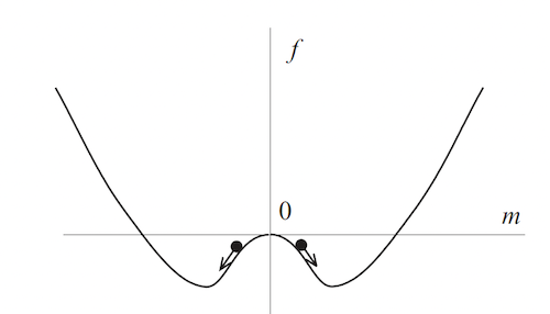
Figure 5: Single pattern retrieval in the Hopfield model
If the Hopfield network is run at some temperature $T>0$, then in equilibrium it will converge to the bottom of one of the two valleys (or pure states), such that the average spin for the equilibrium states is given by the above formula. Note that if $T>0$ then there is more than one such state, in order to retrieve the specific memory, the temperature will have to be gradually reduced to $T=0$.
We can repeat the calculation that we just did for $p$ different $M_{sp}$ vectors with a similar structure, given by $(m,0,…,0), (0,m,0,…,0),…,(0,…,0,m)$ and in each of these cases the $m^\mu=m$ corresponds to the retrieval of the $\mu^{th}$ pattern. Hence we conclude that in a Hopfield network, if the number of patterns is finite, then it is possible to retrieve the appropriate pattern when a noisy version of the pattern is given as the initial condition. This is due to the fact that these patterns correspond to the global free energy minima for the model.
Other Symmetric Solutions for the Hopfield Network
We found a set of $p$ symmetric solutions for the saddle point equations for the free energy of the Hopfield network. Are these the only symmetric solutions that exist? No, there are quite a few more, as first shown by Amit, Gutfreund and Sampolinsky in their pioneering work on the thermodynamics of Hopfield networks. Consider the $p$ dimensional vector given by
\[M_{sp} = m_n(1,1,...,1,0,0,0,...,0)\]where the first $n$ components are ones and the remaining $p-n$ are zero. It can be shown that these are also valid order parameters for the Hopfield network, and for a given value of $n$, there are $p!\over{(p-n)!}$ possible solutions that are equivalent to the one above. These are also symmetric solutions, and the solution in the previous section was actually a special case when $n=1$. The mean field equations for the free energy are given by
\[f_n = {n\over{2}} m_n^2 - {1\over\beta}<\log[2\cosh(\beta m_n z_n)>\] \[m_n = {1\over{n}} < z_n\tanh(\beta m_n z_n) >\]where $< >$ stands for the average over the distribution of the $\xi^\mu_i$ as before and
\[z_n^i = \sum_{\mu=1}^n \xi^\mu_i\]Using similar logic to the one that used for $n=1$, it can be shown that the average spin at the $i^{th}$ node is given by
\[E(\sigma_i) = m_n z^i_n \tanh(\beta m_n z^i_n)\]This equation implies that symmetric solutions with $n>1$ represent states which are equal mixtures of several memories. But what is the relationships between these states? It can be shown that the following ordering exists between the free energies at $T=0$
\[f_1 < f_3 < f_5 <...f_{\infty}...< f_6 < f_4 < f_2\]The even $n$ solutions are unstable at all temperatures, the odd $n$ solutions proliferate as the temperatures falls below $T_c$. Denoting $T_n$ be the threshold below which the $n$ solution is stable, it can be shown that $T_1 = T_c, T_3 = 0.461T_c, T_5 = 0.385T_c, T_7 = 0.345T_c$. The states with $n>1$ were called spurious states at the time Hopfield networks were first proposed since they corresponded to a failure in the retrieval of the memory.
This analysis shows that the solution corresponding to $n=1$ is the most stable one, while the solutions for $n>1$ correspond to local minima of the energy function and represent states that are equal mixtures of several memories. How can we avoid getting stuck in one of these states? The solution is to use simulated annealing, starting at $T$ near $T_c$ and then gradually reducing it. This will enable the system to jump out of the states with $n>1$ by making use of the thermal energy.
Storing an Infinite Number of Patterns
We consider the case in which the number of stored patterns $p$ scales up with N, so that $p=\alpha N$. Using Replica based analysis (see Amit, Gutfreund, Sompolinsky), the following properties have been proven for this system for the case when $T=0$:
- If $\alpha > \alpha_c = 0.138$, only spin glass type solutions exist, which are not correlated with any the memories that we are trying to store.
- For $\alpha <\alpha_c$ a stable solution appears which deviates only slightly from the precise pattern that we are trying to store. The error is about 1.5% at $\alpha=\alpha_c$ and decreases to zero rapidly with decreasing $\alpha$. Hence the system more or less functions as an associative memory at least up to $\alpha\approx 0.14$, in agreement with Hopfield’s original estimate.
Modern Hopfield Networks
More than 30 years after the original Hopfield network was proposed, Krotov and Hopfield introduced a model that has much higher memory capacity. They were motivated by the problem of using the Hopfield network for pattern recognition, in which case the number of stored patterns is much greater than the number of pixels (or nodes) in the image. They proposed the following energy function for their network, now called modern Hopfield networks,
\[H = -\sum_{\mu=1}^K \sum_{i=1}^N\ F(\xi^\mu_i\sigma_i)\]where $F(x)$ is some smooth function. If we restrict ourselves to polynomial functions $F(x) = x^n$, then note that $n=2$ corresponds to the original Hopfield network. Using the same type of crosstalk arguments that were used to compute the capacity of the Hopfield network, they showed that the modern Hopfield network has a capacity of
\[K^{max} \approx {1\over{2(2n-3)! \log N}} {N^{n-1}\over{\log N}}\]for the case in which we want error free retrieval. If we are willing to tolerate a small number of errors in the retrieval, then the capacity is given by
\[K^{max} = \alpha_n N^{n-1}\]where $\alpha_n$ is a constant that depends on the error threshold probability. Hence there is a non-linear relationship between the capacity and the size of the network.
The original Hopfield network was invented as a model for synaptic connections in the brain, which is why it restricted itself to two-node interactions. Clearly the modern Hopfield network involves interactions between more than two nodes and hence is not biologically plausible. Krotov and Hopfield later showed that if we include hidden nodes in the classic Hopfield network, then the resulting energy function for the visible nodes is the same as for the modern Hopfield network, and also all interactions are of the two node type, thus preserving biological plausibility. The addition of hidden nodes increases the number of synaptic connections in the network, which explains the higher capacity of these networks. Hidden nodes are discussed in more detail in the next section on Boltzmann machines and we will see that they are critical to its operation.
In 2017 Demircigil et.al. showed that if the function $f$ is chosen to be exponential, i.e., $F(x) = e^x$, so that the energy function is given by
\[E = -\sum_{\mu=1}^K\sum_{i=1}^N e^{\xi_i^\mu\sigma_i}\]then the capacity of the resulting network is given by
\[K^{max} \approx 2^{N\over{2}}\]Ramsauer et.al. further extended Demircigil et.al.’s work to the case the the $\sigma_i$ are no longer constrained to be $\pm 1$. They made the interesting observation that if the energy function is chosen to be (with $\Sigma = (\sigma_1,…,\sigma_N)$ )
\[E = -lse(\beta,\Xi^T.\Sigma) + {1\over{2}}\Sigma^T.\Sigma + \beta^{-1}\log N + {1\over{2}}M^2\]where $M$ is the largest norm of all the stored patterns and
\[lse(\beta, Z) = \beta^{-1}\log(\sum_{i=1}^N e^{\beta z_i})\]then the update rule for the network is given by
\[\Sigma \leftarrow \Xi.softmax\ (\beta\Xi^T\Sigma)\]which is the same as for the Transformer architecture which is used in LLMs.
From Hopfield Networks to Boltzmann Machines
The discovery of Hopfield networks set off flurry of research activity, and one of the strands led to work that was done by Geoffrey Hinton and Terence Sejnowski, then at CMU and Johns Hopkins respectively. They noticed that the Hopfield network carries out minimization of the energy at $T=0$ in order to retrieve the stored patterns, which can potentially lead to the issue of the system getting stuck in local minima and retrieving the wrong pattern. But what if the minimization were carried out at some temperature $T > 0$ by making use of the Metropolis algorithm? This would cause the system to jump out of local minima with a non-zero probability and thus there would be higher chance that it might end up in a global minima. However a side consequence of making the optimization probabilistic is that the equilibrium configuration at any $T > 0$ is no longer a fixed pattern, but instead it can be one of many patterns governed by the Boltzmann distribution. This seems to go against the idea of using the system as a memory as Hopfield had done. However Hinton and Sejnowski had the brilliant idea that instead of using the system as a memory, use it to model the distribution of the patterns in the data. This could be done if the Boltzmann distribution could be made to approximate the unknown data distribution. Since the Boltzmann distribution is a function of the energy levels, which are in turn a function of the node interactions, the problem reduced to choosing the interactions such that the resulting equilibrium distribution approximated that for the data. Unlike the Hopfield network, the optimal interactions could no longer be written down in a simple manner, but instead had to be learnt from the data. Hinton and Sejnowski came up with a learning algorithm for their system, and they called the resulting network the Boltzmann machine.
When designing his network, Hopfield took a lot of care to make sure that when the system settled into an equilibrium state, its spins were aligned according to one of the patterns it was trying to store. This is no longer the case with the Boltzmann machine. We don’t care about the exact pattern that the network has once it is in equilibrium, but we do care about the constraints and relationships that exist among its spins, and this should follow the same distribution as the training data. This is the critical difference between the Hopfield and Boltzmann networks. The former is concerned with reproducing the exact training pattern, while the latter is concerned about capturing the rules that govern the patterns in the training data.
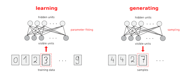
Figure 6: Training and generation phases for a Boltzmann machine
An example of how a Boltzmann machine can be put to use is shown in the above figure. The data consists of handwritten images of numerals from 0 to 9, and these are digitized using a $28 x 28$ grid using 0 for white and 1 for black. Any one of the numerals can be written down as a 784 dimensional vector of ones and zeroes, say $(x_1,…,x_{784})$. The elements of these vectors are distributed according to some unknown distribution $p_X(x_1,x_2,…,x_{784})$ and all we have are samples from this distribution. The Boltzmann machine can be trained using these samples, and it is able to create a representation for this distribution in its node interaction parameters, as shown in the left hand part of the figure. Once the training is complete, it can be used to generate new patterns that confirm to the distribution that it has learnt as shown on the right hand side.
Back in 1983 when Hinton and Sejnowski first thought of using the Hopfield model to capture distributions in the training data, this must have seemed to be somewhat quixotic. But subsequent developments in neural networks have shown that this was a monumental advance in Artificial Intelligence. Indeed lthe latest AI models such as language generating LLMs or image generating models such as SORA are direct descendants that have exploited this fundamental idea. The new models have of course evolved beyond the Boltzmann machine, but they all still generate speech or images by sampling from their representation of some fantastically complex probability distribution that they have learnt from the training data.
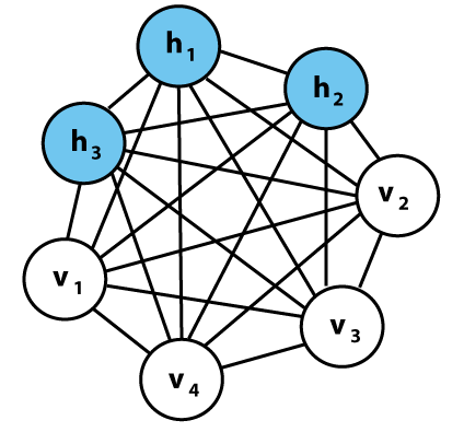
Figure 7: Boltzmann machine with hidden nodes
An example of a Boltzmann machine is shown in the above figure. It has a a fully connected topology as in the Hopfield network, with the ‘spin’ at each node taking on values of 0 or 1. The energy $E$ is also identical to that in the Hopfield network, given by
\[E = -\sum_i\sum_{j\lt i} w_{ij} \sigma_i\sigma_j - \sum_i \sigma_i b_i\]This expression has additional bias parameters $b_i$, which can be though of as a common node to which all other nodes are connected, with interaction strength $b_i$. The symmetric weights $w_{ij}$ and the bias’s $b_i$ are real numbers, that can be either positive or negative, and have to be learnt from the training data, and in this respect the model differs from the Hopfield network. If $\Delta E_k$ is the difference in energy levels between the $k^{th}$ node being 1 or 0, then it can be shown that
\[\Delta E_k = h_k = \sum_i w_{ki}\sigma_i + b_k\]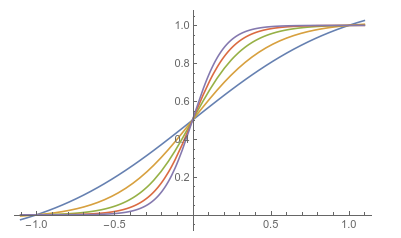
Figure 8: The sigmoid function for various values of $T$
The Boltzmann machine uses a probabilistic rule called Gibbs sampling, which is derived from the Glauber rule, to update its spins. This rule says that the $k^{th}$ node should be turned on (or its spin set to $+1$) with probability given by $p_k$ given by
\[p(\sigma_k = 1) = p_k = {1\over{1 + \exp(-\beta h_k)}}\]and this is irrespective of its previous state. As $T\rightarrow 0$, this rule becomes the Hopfield rule, while as $T\rightarrow\infty$ the assignment becomes completely random. The above figure plots $p_k$ for various values of $T$.
There is another architectural subtlety that has to be taken care of. In the figure for the Boltzmann machine we can see that the seven nodes have been divided into two classes, namely the visible nodes $v = (v_1,v_2,v_3,v_4)$ and the hidden nodes $h= (h_1,h_2,h_3)$. The visible nodes are the interface between the network and the outside world, during training they are clamped into specific states determined by the training data. The hidden nodes are never clamped, and the additional weights (or interactions) that they introduce into the network help expand the scope of the environment probability distributions that can be captured by the model. For example if there are $V$ visible nodes and $H$ hidden nodes, then there are ${(V+H)(V+H-1)\over 2}$ parameters that the network can adjust vs just ${V^2\over 2}$ otherwise.
The weights of the connections to the hidden nodes can be used to represent complex interactions that cannot be expressed as pairwise interactions between the visible nodes alone. The hidden nodes are where the network can build its own internal representation of the data. This idea has stood the test of time, indeed modern neural networks feature hundreds of hidden layers. Even Boltzmann machines were modified a few years later with multiple hidden layers, to form what are called Deep Boltzmann machines.
Using our knowledge of thermodynamics, it follows that if this system is allowed to evolve, then it will eventually settle into an equilibrium, such that the probability $p(v,h)$ that the system is in state $(v,h)$, where $v=(v_1,…,v_V)$ and $h=(h_1,…,h_H)$ are vectors of the visible and hidden node values, is given by the Boltzmann distribution.
\[p(v,h) = {1\over Z} \exp[-\beta E(v,h)]\]where $E(v,h)$ is the energy of the $(v,h)$ state. We can therefore control the probabilities of network states by controlling their energies. We are really interested in the marginal distribution of the visible nodes, which is given by
\[p(v) = \sum_{[h]} p(v,h) = {1\over Z} \sum_{[h]} \exp[-\beta E(v,h)]\]where the sum is over all possible permutations of the spins of the hidden nodes.
Training the Boltzmann Machine
How can we determine the interaction weights $w_{ij}$ (and biases $b_i$) in a Boltzmann machine? Assume that the (unknown) probability that the environment, as represented by the $V$ elements of the training data vector, is in state $v$ is given by $q(v)$. Note that there are $2^{V}$ probabilities that are needed to fully specify $q(v)$ while there are at most ${(V+H-1)(V+H)\over 2}$ weights and $(V+H)$ thresholds. However if there are some regularities in the environmental distribution, then perhaps it could be exploited by the model to approximate it using a fewer number of parameters.
Assume that we have $N$ training samples with possible values $v(1),…,v(N)$ where $v(i)$ is a vector $v(i) = (v_1(i),…,v_V(i), i=1,…,N$ where $V$ is the number of visible nodes. Assuming that the training dataset is made up of statistically independent samples, the probability for the entire training set is given by
\[p(V) = \prod_{k=1}^N p(v(k))\]We will now use the principle of Maximum Likelihood to get estimates of the parameters $(w_{ij}, b_{i})$. It states that the best estimates, say $w_{ML}, b_{ML}$ are given by
\[w_{ML} = arg\ max_{w} p(V) = arg\ max_{w} \log p(V)\ and\ b_{ML} = arg\ max_{b} p(V) = arg\ max_{b} \log p(V)\]The log function has been used since it simplifies the calculations, and since it is monotonically increasing, it does not affect the maximal values.
It can be shown that the maximum likelihood estimate of the weights results in a probability distribution $p(v)$ over the visible states, such that Kullback-Leibler distance $KL(q\vert\vert p)$ between the environmental distribution $q$ and the model distribution $p$ given by
\[KL(q\vert\vert p) = \sum_{v} q(v)\log{q(v)\over p(v)}\]is minimized.
It follows from the independence of samples that
\[w_{ML} = arg\ max_{w} \log(\prod_{k=1}^N p(v(k)) = arg\ max_{w} \sum_{k=1}^N \log p(v(k))\]and similarly for $b_{ML}$. Define $L(w)$ as
\[L(w) = \sum_{k=1}^N \log p(v(k))\]By the law of total probability
\[p(v(k)) = \sum_{[h]} p(v(k),h) = {1\over{Z}} \sum_{[h]}\exp[-\beta E(v(k),h)]\ where\ Z = \sum_{[x]} \exp[-\beta E(x)]\]In this formula $(v(k),h)$ is the equilibrium state of the Boltzmann machine when the visible nodes are clamped at $v(k)$ while the hidden nodes are allowed to run freely, $x=(v,h)$ is the equilibrium state of the Boltzmann machine when both the visible and hidden nodes are allowed to run freely, and the sums are over all possible permutations of the free nodes. It follows that
\[L(w) = \sum_{k=1}^N \log({1\over{Z}} \sum_{[h]} \exp[-\beta E(v(k),h)])\] \[= \sum_{k=1}^N \log( \sum_{[h]} \exp[-\beta E(v(k),h)]) - \log(\sum_{[x]} \exp[-\beta E(x)] )\]As per the Maximum Likelihood principle, the best estimates of $(w_{ij}, b_i)$ are those for which $L(w)$ is at a maximum. Unfortunately it is not possible to find the best parameters analytically, so we are going to use the gradient ascent algorithm, which iterates from a starting value of $(w_{ij}, b_i)$ by using the equation
\[w_{ij} \leftarrow w_{ij} + \eta {\partial L(w)\over{\partial w_{ij}}}\ \ \ b_i \leftarrow b_i + \eta {\partial L(w)\over{\partial b_i}}\]where $\eta$ is called the learning rate parameter whose value can be adjusted to aid the convergence to the maximum value. In order to implement this we have to compute the derivative
\[{\partial L(w)\over{\partial w_{ij}}} = \sum_{k=1}^N {\partial\over{\partial w_{ij}}}\log(\sum_{[h]} \exp[-\beta E(v(k),h)]) - {\partial\over{\partial w_{ij}}}\log(\sum_{[x]} \exp[-\beta E(x)])\]After some simplification, this can be written as
\[{\partial L(w)\over{\partial w_{ij}}} = \beta\sum_{k=1}^N(\sum_{[h]} p(v(k),h)]\sigma_i \sigma_j - \sum_{[x]} p(x) \sigma_i \sigma_j)\]Define
\[< \sigma_i \sigma_j >_{data} = \sum_{k=1}^N\sum_{[h]} p(v(k),h)\sigma_i \sigma_j\]This is the correlation between the spins $\sigma_i$ and $\sigma_j$ when the visible nodes in the network are clamped to the training vector $v(k)$ and hidden nodes are allowed to run freely. Also define
\[< \sigma_i \sigma_j >_{model} = \sum_{k=1}^N\sum_{[x]} p(x) \sigma_i \sigma_j\]This the correlation between the spins $\sigma_i$ and $\sigma_j$ when the network is allowed to run freely. The derivative can then be written as
\[{\partial L(w)\over{\partial w_{ij}}} = \beta(< \sigma_i \sigma_j >_{data} - <\sigma_i \sigma_j >_{model})\]Using this formula, it follows that the Boltzmann Machine can be trained by using the gradient ascent rule
\[w_{ij}\leftarrow w_{ij} + \eta {\partial L(w)\over{\partial w_{ij}}} = w_{ij} + \eta\beta (< \sigma_i \sigma_j >_{data} - <\sigma_i \sigma_j >_{model})\]and for the biases
\[b_i\leftarrow b_i + \eta {\partial L(w)\over{\partial b_i}} = b_i + \eta\beta (< \sigma_i >_{data} - < \sigma_i >_{model})\]Note that both these correlations have to be measured after the network has attained equilibrium.
Based on these calculations there are two phases to the operation of the Boltzmann machine:
(1) Positive phase: In this phase, the network operates in its clamped condition under the direct influence of the training sample. The visible nodes are all clamped onto specific states determined by the environment while the hidden nodes are allowed to run freely.
(2) Negative phase. In this second phase, the entire network is allowed to run freely, and therefore with no environmental input. The initial states of the nodes are set randomly. The probability of finding it in any particular global state after each reaches equilibrium depends on the energy function.
The training dataset is divided in batches of smaller size, called mini-batches, and the gradient is computed over each mini-batch. The weights and biases are initialized using random numbers, with small values chosen from a zero mean Gaussian with a standard deviation of about $0.01$.
Here is the complete algorithm: Initialize
\[pp_{ij} = 0,\ pp_{i0} = 0,\ pn_{ij} = 0,\ pn_{i0} = 0\]For $k=1,2,…,N$ do the following:
Positive Phase: The system is initialized to the starting for the visible units clamped to $v(k)$ and the hidden units are chosen at random, 0 or 1. Allow the system to evolve using Gibbs sampling, until thermal equilibrium is reached. Store the statistics
\[pp_{ij}^{new} = pp_{ij}^{old} + 1\ if\ \sigma_i \sigma_j = 1\ and\ pp_{ij}^{old}\ otherwise\]and for the biases
\[pp_{i0}^{new} = pp_{i0}^{old} + 1\ if\ \sigma_i = 1\ and\ pp_{i0}^{old}\ otherwise\]Negative Phase: All the nodes in the system, both visible and hidden, are initialized at random to 0 or 1. Allow the system to evolve using Gibbs sampling, until thermal equilibrium is reached. Store the statistics
\[pn_{ij}^{new} = pn_{ij}^{old} + 1\ if\ \sigma_i \sigma_j = 1\ and\ pn_{ij}^{old}\ otherwise\]and for the biases
\[pn_{i0}^{new} = pn_{i0}^{old} + 1\ if\ \sigma_i = 1\ and\ pn_{i0}^{old}\ otherwise\]Normalize
\[{\overline pp}_{ij}^{new} = {pp_{ij}^{new}\over N},\ {\overline pp}_{i0}^{new} = {pp_{i0}^{new}\over N}\] \[{\overline pn}_{ij}^{new} = {pn_{ij}^{new}\over N},\ {\overline pn}_{i0}^{new} = {pn_{i0}^{new}\over N}\]Finally the weights and biases are adapted according to
\[w_{ij}\leftarrow w_{ij} + \eta\beta({\overline pp}_{ij} - {\overline pn}_{ij})\] \[b_i\leftarrow b_{i} + \eta\beta({\overline pp}_{i0} - {\overline pn}_{i0})\]Note that greater correlation between the spins at nodes $i$ and $j$ when the visible nodes are clamped, leads to an increase in the weight $w_{ij}$, which is another instance of Hebb’s rule, though in this case the rule arises naturally through the optimization process (unlike the Hopfield network where it was put in by design). On the other hand when the visible nodes are not clamped, then any increase in the correlation between the spins at nodes $i$ and $j$ leads to a decrease in the weight value $w_{ij}$.
Restricted Boltzmann Machines
The Boltzmann machine suffers from the problem that it takes too long to train. This is a result of the fact that training require the system to settle down into equilibrium, in both the positive and negative parts of the training cycle, and this time increases exponentially with the number of nodes. The Restricted Boltzmann Machine or RBM was designed with the objective of making the training more efficient.
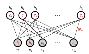
Figure 9: A Restricted Boltzmann Machine
The connections in a RBM are restricted to those between the visible and hidden units, as shown in the above figure which considerably simplifies both the training as well as inference phases in the system. The energy in a RBM can be written as
\[E(v,h) = -\sum_{i=1}^H\sum_{j=1}^V w_{ij} h_i v_j - \sum_{i=1}^H b_i h_i - \sum_{j=1}^V c_j v_j\]The benefit of having this bi-partite structure is that that hidden node spins are independent given the visible node spins and vice versa, i.e.,
\[p(h\vert v) = \prod_{i=1}^H p(h_i\vert v)\ and\ p(v\vert h) = \prod_{j=1}^V p(v_j\vert h)\]where
\[p(h_i = 1\vert v) = sig(\sum_{j=1}^V w_{ij} v_j + c_i)\ and\ p(v_j = 1\vert h) = sig(\sum_{i=1}^H w_{ij} h_i + b_j)\]where $sig(.)$ stands for the sigmoid function $sig(x) = {1\over{1+\exp(-x)}}$. The conditional independence property simplifies the Gibbs sampling since the new state for all the nodes in a layer can be sampled in parallel. Thus a complete sampling sweep through all the nodes can be performed in two steps: Sample a new state $h$ for the hidden nodes based on $p(h\vert v)$ and then sample the a state $v$ for the visible layer based on $p(v\vert h)$.
It is possible to obtain an expression for the distribution $p(v)$, as follows
\[p(v) = \sum_h p(v,h) = {1\over {Z}} \sum_{[h]} \exp[-E(v,h)] = {1\over{Z}}\prod_{j=1}^V \exp(b_j v_j) \prod_{i=1}^n (1 + \exp[c_i + \sum_{j=1}^m w_{ij} v_j])\]This expression shows how the parameters $(w_{ij}, b_i, c_i)$ combine together to generate the visible layer probabilities. It can be shown that any discrete distribution on $(0,1)^V$ can be modeled arbitrarily well by an RBM with $V$ visible and $k+1$ hidden units, where $k$ denotes the cardinality of the support set for the distribution in the training dataset, i.e., the number of elements in $(0,1)^V$ that have a non-zero probability of being observed.
The Contrastive Divergence (CD) Algorithm
Recall that weights in the regular Boltzmann machine were updated according to
\[w_{ij}\leftarrow w_{ij} + \eta\beta({\overline pp}_{ij} - {\overline pn}_{ij})\]The first term ${\overline pp}_{ij}$ can be simplified by noting that once the visible units are clamped, the equilibrium value of the hidden units can be computed in a single pass due to the independence property noted above. Let us denote the resulting correlation by $[v_i h_j]_0$.
In order to obtain the second term ${\overline pn}_{ij}$ term we can carry out the following procedure:
- Starting with a training data vector on the visible units, and update all the hidden units in parallel.
- Update all the visible units in parallel to get a ‘reconstruction’ of the original training data.
- Update all the hidden units again.
Denoting the correlation after $k$ cycles of this procedure as $[v_i h_j]_k$, the weight update equation can be written as
\[w_{ij}\leftarrow w_{ij} + \eta\beta([v_i h_j]_0 - [v_i h_j]_{\infty})\]Geoff Hinton proposed that a good approximation to the gradient can be obtained after stopping the reconstruction procedure after $k$ steps, so that
\[w_{ij}\leftarrow w_{ij} + \eta\beta([v_i h_j]_0 - [v_i h_j]_k)\]This resulting training algorithm is called k-step contrastive divergence, or CD, algorithm and works quite well in practice, in fact in many cases it works even for $k=1$. This algorithm works by shaping the energy landscape of the visible nodes of the RBM such that the energy is lowered for the spin configurations that correspond to patterns in the training data, and is raised for patterns that lie close to the training data. In other words, it creates deep energy valleys in the surface area surrounding the patterns in the training data set. Here is an intuitive explanation of how it does that:
- In order to reduce the KL distance between the actual data distribution $q(v)$ and the distribution $p(v)$ as predicted by the RBM, the maximum likelihood function $L(w)$ has to maximized (here $w$ represents the weights and biases in the network).
- $L$ is maximized by doing the iteration
- In order to maximize $L(w)$ we need to maximize the positive term $[v_i h_j]_0$ and minimize the negative term $[v_i h_j]_k$. Maximizing the positive term is the same as maximizing the correlation between the training data set and the spins computed in the hidden layer. Minimizing the negative term is the same as reducing the correlation between visible spins that are not in the training data, and the spins in the hidden layer (both of these as computed after $k$ iterations) . But remember that the visible spins after $k$ iterations are obtained by starting from a training data vector, and then doing $k$ iterations. Thus the resulting spin will tend to be close to the original training vector.
- From the expression $E = - \sum_v\sum_h w_{ij} h_i v_j$ for the energy, it follows that higher values of $w_{ij}$ lead to lower energy if the training data and hidden layer spins are more correlated AND the spins that are part of the nearby vectors are less correlated with the hidden layer. Hence as the training progresses, the energy levels for spins in the training dataset go down while the energy levels for spins that are in the vicinity of the training dataset go up. This is in contrast to the non-CD way of training in which the negative phase is initialized with a random spin vector, and this makes the convergence happen much slower because we are increasing the energy levels at random points in the energy landscape vs close to the training data points.
Thermodynamics of the RBM
Unlike the Hopfield network, RBMs present a number of challenges which has made their analysis using tools from statistical mechanics difficult. In particular:
- We can no longer assign a probability distribution to the data samples (recall that these were set to the Bernoulli distribution in the Hopfield case), since the whole purpose of an RBM is to be able to approximate some unknown data distribution.
- The weights $w_{ij}$ can no longer be assumed to independent, since in practice it has been found that there exhibit a strong correlation in a trained RBM.
Some good progress in this area was made by Decelle, Fissore, Furtlehner, who were able to an analysis of RBMs without making any of these two assumptions (also see Decelle and Furtlehenr for a good survey of recent work in this area). They did so by modeling the structure of the weights $w_{ij}$ by using singular value decomposition (SVD) theory, whereby the weight matrix can be expressed in a form that is similar to that in the Hopfield model. Under this assumption, they used replica theory to obtain an expression for the free energy and obtained solutions for the replica symmetric case. Among other things they showed the following:
- Just as in other spin glass type systems, the behavior of the RBM can be classified into paramagnetic, ferromagnetic and spin glass phases. When the RBM is operating properly, it is in ferromagnetic phase.
- When an RBM starts to train its weights are initialized to random values and as a result it is in the paramagnetic phase. As the training progresses the weights change and this causes the RBM to cross over to the ferromagnetic portion of the phase space.
- The number of pure states or valleys in the ferromagnetic phase can be identified by solving the equivalent of the TAP equations for RBMs, and they act as attractors for the visible states. At the equilibrium point in a valley, the visible nodes can be in one of many possible configurations, and these correspond to variations in an image datapoint that RBM has learnt.
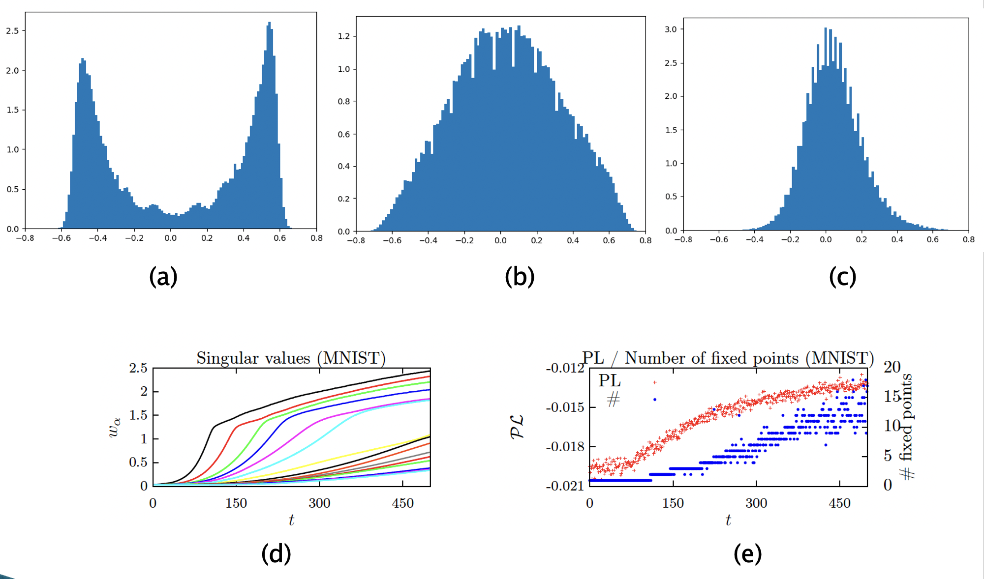
Figure 10: Changes in the weight matrix as the RBM undergoes training
A great deal of insight can be obtained into the learning behavior of RBMs by analyzing the evolution of the weight matrix $w_{ij}$ while the RBM is undergoing training. There are two ways to look at this matrix: (1) The values of the weights themselves, and the distances between them, (2) By doing a singular value decomposition of the $w_{ij}$ matrix, given by
\[W = U\Sigma V^T\]where $U$ and $V$ are orthogonal matrices and $\Sigma$ is a diagonal matrix whose elements are the eigenvalues for $W$ (also called the modes of $W$).
The above figure shows experimental data collected while the RBM was being trained on MNIST data. The top part of the figure plots the histogram of the distances between the weight values for three different cases during the course of training. When the training starts the weights are initialized to random Gaussian values and hence the histogram of distances is also Gaussian and centered at zero which puts the RBM in the paramagnetic phase. As the training proceeds the RBM enters the ferromagnetic phase and the eigenvalues assume a structure in which there is a dominant mode and this results in high positive or negative inter-weight distance as shown in part (a). This is also seen by directly plotting the eigenvalues, as shown in part (d), we can see that the ‘blue’ eigenvalue has assumes larger values while the others are still small. The resulting samples from the RBM don’t look very different than the ones that were used for training. Part (b) shows the inter-weight values after further training has taken place. Part (d) of the figure shows that many more modes have emerged and the histogram of distances is much broader, but the generated samples still correspond closely to the training data with not much variation. After further training the RBM becomes fully trained and starts to generate a variety of good samples. In this case the eigenvalues are close to each other as seen in part (d) of the figure, while the inter-weight distance is still centered at zero, but with a much smaller variance, as shown in part (c). Part (e) of the figure shows the number of fixed point of the mean field equations for the RBM, and these correspond to the number of patterns that it can produce. We can see that starting from zero in the paramagnetic phase, the number of fixed points progressively increases as the training goes on, and it actually exceeds the number of MNIST classes if continued for a long time.
Recent Developments in Boltzmann Machines
The classic Boltzmann Machine described here suffers from two issues:
- Convergence Time: Both the training and inference phases of the Boltzmann Machine involve waiting for the system to reach convergence before we can sample from it. This time can be quite excessive as the number of nodes in the system increases, and the cause for this can be traced to the high energy barriers that exist between valleys representing the training data.
- Inefficient Sampling: Since the Boltzmann Machine is simulated on a digital computer, we are forced to use Gibbs sampling to update its state. Unfortunately Gibbs sampling updates just one node at a time, and this can’t be parallelized using our current technology (GPUs are not able help here). This problem is somewhat alleviated with the RBMs, but in the process we lose some computational power in the system.
Both these issues are related to the fact that the Boltzmann Machine is an inherently probabilistic system which makes use of thermal randomness in its operation, and digital computers are not the best platform for them. In recent years several research groups have begun to tackle this problem by advancing both the theory of Boltzmann Machines as well as coming up with new computational devices that can implement them more efficiently, this is covered in Part 3.