Energy Based Models Part 1: Ising and Spin Glass Models
Contents
- Introduction
- Statistical Mechanics basics
- The Boltzmann distribution
- Free energy
- Models for magnetism
- Model for paramagnetism
- Ising model in one dimension
- Ising model in 2 or more dimensions: Phase transitions
- Simulating spin systems
- The Landau theory of phase transitions
- Spin Glass models: Randomized interactions
- The Sherrington-Kirkpatrick (SK) model
- Order parameters
- The replica method and replica symmetry breaking
- The p-spin spherical spin glass model (PSM)
- Simulated Annealing
Abstract
This and the following two posts are a deep dive into Energy Based Models or EBMs. The original EBMs were proposed by physicists in the late 19th century, and form the backbone of the theory of statistical mechanics. So we will start with statistical mechanics and the basics of how concepts such as entropy were discovered. We then apply this theory to a model for magnetism called the Ising model. This takes us to the physics behind phase transitions, the simplest example of this being when a ferromagnetic material becomes magnetized as the temperature is reduced. The Ising model can be generalized to the case when the nodes in the system interact with each other in more complex ways, and this takes us to spin glass models and the phenomenon of continuous symmetry breaking.
The present generation of neural network models can be traced to a spin glass inspired EBM called the Hopfield network that was proposed in the early 1980s, and this was soon followed by another more influential EBM called the Boltzmann Machine. Until about 2010 these were the only games in town as far as neural networks were concerned, however soon after that people discovered how to train very large non-EBM models by resolving the problems with the backpropagation training algorithm. Since then EBMs have taken a somewhat of a backseat in AI systems, especially since a way to scale them up hasn’t been found. However very large non-EBM systems such as LLMs have run into another problem, which is that of excess energy consumption. Indeed, a large portion of new power capacity being added to our energy grids is being driven by the demand from LLMs. This has caused some people to look at alternative designs that are less power hungry, and perhaps EBMs have a role to play here. As I was putting the finishing touches to this post, a start-up called Extropic announced a new chip that works using EBM principles, and the claim is that it reduces power consumption by four orders of magnitude.
This post is divided into three parts: Part 1 covers the fundamentals of statistical mechanics and EBMs, while Part 2 is on Hopfield Networks and Boltzmann Machines. In Part 3 (in preparaton) I will look at more recent developments in this area, including Extropic, and what the future holds for EBMs.
Introduction
The steam engine was invented in the late 1700s, the inventors were brilliant tinkerers who made this advance solely through smart experimentation. But soon after, the question arose about how to make a better engine, and in particular how could one get the most work out of it. This question led to the launch of the science of thermodynamics, and the biggest early contribution was made by the great French engineer Sadi Carnot. Carnot came up with a model for an ideal engine, and showed that the efficiency of any engine is upper bounded by that of his model. This was the genesis of the second law of thermodynamics, also called the law of entropy and soon after this was joined by the first law, called the law of conservation of energy, with the efforts of Count Rumsfeld, James Joule and others. The concepts of the flow of heat and that of entropy were introduced as part of these laws, but it was a big mystery as to what exactly these were.
The first efforts in coming up with an explanation was made in the latter half of the nineteenth century, and the names associated with this are that of James Clerk Maxwell, and more importantly that of the Viennese physicist Ludwig Boltzmann. They started from the single hypothesis, that all matter is made up of tiny particles called atoms, and through a brilliant series of mathematical investigations they were able to explain not just the true nature of heat as the thermal jiggling of atoms, but also that of the mysterious entropy, and a lot more besides. In the process they founded the science of statistical mechanics, and launched a revolution in physics whose effects are being felt even to the present day. Statistical mechanics connected the microscopic properties of atoms, mainly their energy and the way they interact with each other, with macroscopic quantities that we can measure, such as temperature, entropy, pressure, specific heat etc. The biggest mystery that the new science was able to explain was the true nature of phase transitions, such as ice melting or a piece of iron getting magnetized. These are sudden changes in the physical properties of matter which cannot be explained without considering the joint behavior of a large number of interacting particles.
Classical Newtonian mechanics is a deterministic theory. Once we know the initial conditions for a system of particles, it was thought that it should be theoretically possible to predict the future behavior of the system by using Newton’s Laws of motion. The conceptual leap that statistical mechanics made, was to give up on making exact predictions when the number of particles is very large and this was done by basing the new science on the mathematics of probability theory. The theory embraced the idea that all predictions for these systems should be statistical in nature, hence the results of the theory were in the form of statistical quantities such as averages and distributions.
The randomness in these systems that requires the use of statistical methods is a result of thermal motion, and things become more random as the temperature increases. Boltzmann’s great insight was the realization that this randomness could be captured in terms of a probability distribution, now called the Boltzmann distribution, given by
\[p_i = {e^{-\beta E_i}\over{\sum_j e^{-\beta E_j}}}\]where $p_i$ is the probability that the system is in the $i^{th}$ state, $\beta={1\over T}$ is the inverse temperature and $E_i$ is the energy of the $i^{th}$ state. This is one of the most important formulae in all of physics and underlies statistical mechanics. The definition of a state depends on the physics of the system under consideration: For example, for a box of gas it would be the number of molecules moving with a certain velocity, for a magnet it would be the number of atoms with spins pointing in a certain direction etc. A few decades after Boltzmann, probability once again entered physics by way of quantum mechanics. In statistical mechanics probabilities reflect the fact that we have an imperfect knowledge about the state the system is in, but is that the case for quantum mechanics too? In other words does a quantum system such as an electron have internal microstates, and the lack of knowledge of those states leads to uncertainties when we make measurements. A lot of people, including Einstein, though so, and the internal microstates of a quantum system were called hidden variables. However, in 1960s Joseph Bell proved that there are no such hidden variables in quantum theory, and hence quantum probabilities are fundamentally different than those in statistical mechanics.
Statistical mechanics also led to a precise definition for the entropy of a system. Entropy had been introduced in the mid-1800s by the German scientist Rudolf Clausius as way of restating Carnot’s results for the efficiency of the ideal steam engine, and it is something that could be measured macroscopically, but its true nature remained a mystery. Boltzmann showed that entropy was a measure of our ignorance of the state of the system, and gave a formula for entropy
\[S = -\sum_i p_i\log p_i\]where $p_i$ is from the Boltzmann distribution, so that greater uncertainty about the state of the system led to higher entropy. This implied that if we have a more information about the system state then the entropy would be lower. This definition did not entirely clear up the matter, since it implied that entropy was not an objective property of the system, but instead was connected to the observer’s knowledge about the system. There were paradoxes such as that of Maxwell’s Demon that were thought up to illustrate this point, and this is where things stood until Claude Shannon came along.
In the 1940s Shannon was looking for a measure of our ignorance about the contents of a message, and he hit upon a formula that was precisely the same as Boltzmann’s definition of entropy (though Shannon was not aware of it at that time). Shannon actually derived the formula for entropy by purely probabilistic reasoning, by looking for a measure of the amount of uncertainty in a probability distribution and this definition was applicable to any distribution whatsoever, whether it arose in statistical mechanics or information theory. This led to a reformulation and re-thinking of statistical mechanics, in which entropy was now the primary quantity, and it was shown that the rest of the statistical mechanics could be derived starting from this. The only physical assumption required was an enumeration of the states of the system and their energy levels, the rest of it was purely probabilistic analysis. Hence in some sense statistical mechanics was reduced to a sub-branch of probability theory.
One of the mysteries that statistical mechanics cleared up was that of phase transitions and the emergence of spontaneous order. This is the phenomenon observed when the physical properties of a collection of particles suddenly change, either as a result of variation of temperature or pressure. For example, when water suddenly turns to steam at its boiling point or into ice at its freezing point. In the 1870s Van der Waals showed that phase transitions in a gas could be explained using statistical mechanics if we add a force of attraction between particles that are near each other. Thus he introduced the important concept of an interacting particle system into statistical mechanics. Needless to say phase transitions don’t occur at the level of individual particles, but somehow a collection of particles collectively exhibit behavior which are not seen at the microscopic level.
In the 1920s the physicist Wilhelm Lenz and his student Ernst Ising came up with a model for ferromagnetism using statistical mechanics. The significance of this model is that it explained magnetism as a result of a phase change in the material. The Ising model, as it is now called, has become the most important model in statistical mechanics since it is reasonably simple, but at the same time exhibits complex phase behavior. In the next few decades more detail was added to this model, ultimately resulting in statistical field theory which was introduced by the great Russian physicist Lev Landau in the 1940s. A final explanation for certain aspects of phase transitions had to wait until the 1970s with the renormalization group theory proposed by the American physicist Kenneth Wilson.
Some of the biggest advances in physics in the last 100 years have been a result of applying statistical mechanics to areas which at first glance are remote from its origins as a theory of gas particles. In addition to the Ising model for ferromagnetism, they include the following:
- The electromagnetic radiation within a closed chamber can be considered to be a type of gas, but made up of light photons rather than atoms, and its physics can be analyzed using the methods of statistical mechanics. This is precisely what Max Planck did in 1901, when he noticed that in order to get agreement with experimental data, the photon’s energy levels have to come in discrete chunks, thus launching the science of quantum mechanics. In the 1920s Satyendra Nath Bose improved upon this model for radiation, which led to Bose-Einstein statistics in quantum theory.
- Statistical mechanics can be applied to solids as well as to gases or liquids, and Albert Einstein did so in 1907 to understand the specific heat behavior with temperature for a solid. He did so by modeling it as a system of fixed particles, each of which is a simple harmonic oscillator with discrete energy levels. This model successfully predicted the experimental observations in the high temperature range. The low temperature part was corrected by Peter Debye a few years later, with his theory of phonons.
- Statistical mechanics has been used to create a model for the phenomena of electrical conduction in metals. This is done by regarding the metal as a sort of closed box that contains a cloud of electrons. The initial analysis of this model was done by Paul Drude before the advent of quantum mechanics, and later Arnold Sommerfield made the quantum corrections in 1927 using the newly proposed theory of Fermi-Dirac statistics.
- Phenomenona such as superconductivity and superfluidity were explained using the tools from statistical mechanics.
In the last few decades statistical mechanics has been extended to non-traditional systems, and one of these is to a type of material called a spin glass. These are made in the lab by creating an alloy of a conducting material such as copper and small amounts of a magnetic materials such as iron. When the temperature is decreased, the magnetic material tries to align all its spins in the same direction, but is prevented from doing so by the surrounding conductor. This complicates the interaction between nearby spins, since a spin can be simultaneously subject to forces that try to align it in opposite directions, which is a phenomenon called ‘frustration’. Frustration causes the spin orientation of an atom to be randomly oriented even at very low temperatures, and one consequence of this is that the phase change behavior of these materials is very different than that for ferromagnetic materials. Whereas a ferromagnet only has two phases, a spin glass exhibits hundreds of thousands of phases as the temperature is progressively reduced. It turns out that this is a very interesting property that has been exploited by both biological systems, as well as man-made systems that mimic biological systems such as neural networks. In order to understand why this is the case, consider the following:
- Complex biological systems can be modeled as spin glasses. For example Stuart Kauffmann has pointed out that in molecules that are a linear sequence of smaller molecules, such as proteins made from amino acids or DNA made from nucleotides, the smaller units interact in complex ways with each other, which is similar to spins in a spin glass. The same goes for interactions between basic units such as neurons in an artificial neural network. Kauffman has argued that the order seen in biological systems emerges to large extent as a result of laws of statistical mechanics, and Darwinian natural selection then acts on this substrate to create living cells.
- The many phases in a spin glass can be used to create an information structure which can be utilized for various functions. For example the frozen spin patterns can be used as a memory, so the spin glass becomes a model for associative memory as John Hopfield first pointed out.
Spin glass models first appeared in the mid-1970s and these were extensions to the classical Ising model for ferro-magnetism. The Edwards-Anderson model was the first one that was proposed, followed by the Sherrington-Kirkpatrick or SK model which proved to be more versatile and easier to analyze and has served as the most popular spin glass model since then. A full understanding of the phase transition behavior of the SK model had to wait until the mid 1980s, and the name most closely associated with this is that of the Italian physicist Giorgio Parisi. He showed that the SK model can exist in a very large number of phases that are organized by energy in an hierarchical tree like fashion at low temperature, and sometimes it can be in multiple phases at the same time, a little bit like how water can exist in the liquid and gas phase simultaneously at its boiling point.
Spin glasses by themselves haven’t become commercially important as materials, but the models that were built to explain their behavior had an unexpected side effect. They inspired the neural network models that were proposed in 1980s, initially by John Hopfield at Caltech, and later by Geoffrey Hinton and his collaborators. Hopfield regarded his network as a type of spin glass, more precisely as a modified SK model, and showed that the system can be made to function as an associative memory. Hopfield’s great insight was the realization the interaction between spins in his model could be chosen in a manner such that it resulted in as many phases as there are memories to the stored, and moreover the equilibrium spin configuration in each phase corresponds with one of the stored memories. Hence if the system is initialized in a state that is near a stored memory, then it gradually settles into an equilibrium configuration that corresponds to that memory.
Hinton and Sejnowski were inspired by Hopfield’s work, but they asked a different question. Instead of trying to remember the exact bit patterns, which is what the Hopfield network does, what if a network could be used to generate samples from the (unknown) probability distribution that the training data was drawn from. This is a very important problem in practice, for example consider the following: We have a bunch of N dimensional training data samples $(x_1,…,x_N)$ drawn from some unknown probability distribution $q(x_1,…,x_N)$. For example a sample could be an N pixel image, with each pixel assuming either black or white values. If the network can be trained to learn this probability distribution, then it can be used it to generate new samples and thus the network becomes a generator of new images similar to those in the training dataset. This was the very beginning of the field of generative AI which has assumed such gigantic importance in the present day, with LLMs being the prime example. Hinton and Sejnowski named their network the Boltzmann machine, the reason being that the equilibrium Boltzmann distribution $p$ of the spins in their network served as an approximation to the unknown probability distribution $q$. How were they able to accomplish this? They did it introducing the idea of learning the inter-node interactions (or weights) from the training data such that the ‘distance’ between the distributions $p$ and $q$ is minimized. The neural networks that that we use today are a direct descendant of these early models and use similar principles.
Boltzmann Machines embody an important principle: By introducing stochasticity into an algorithm (in this case the Hopfield Network), the resulting system becomes much more powerful. Modern machines learning systems have begun to introduce random noise as part of the training, a good example of this is diffusion models which are the state of the art way to generate images and video. In some sense the diffusion model can be considered to be a more complex form of the Boltzmann Machine, and this correspondence is explored fully in Part 3 of this article. Biological systems also exploit randomness in their operation since they operate in a thermodynamic environment in which thermal noise is ever present. But at the same time they are much more powerful than the silicon systems that we have invented so far, and they are able to do their job with a much lower expend of energy. There is a new discipline called Thermodynamic Computing that aims to make machine learning systems more energy efficient by exploiting the thermodynamic properties of the devices used to implement them, and this is also covered in Part 3.
Statistical Mechanics Basics
Suppose a quantity $x$ can assume the discrete values $x_i, i=1,2,..n$ with the unknown probabilities $p_i$, and all that is known is the expectation $f_{av}$ of the function $f(x_i)$, so that
\[f_{av} = \sum_i p_i f(x_i)\ \ \ \ \ \ \ \ \ \ \ \ \ \ \ \ \ \ \ \ \ \ \ \ \ \ \ \ \ \ \ \ \ \ \ \ \ \ \ (1)\]On the basis of this information alone, what are the best estimates of the probabilities $p_i, i=1,2,…n$? This is a classic problem in probability theory, and in order to solve it we need a measure of our ignorance of the probability distribution. If we have such a measure, that quantifies ignorance or uncertainty, then the best estimates for $p_i$ would be those that maximize this quantity.
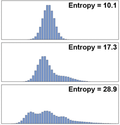
Figure 1: Illustrating the change in entropy with the spread of the probability distribution
How can we quantify the amount of uncertainty in a discrete probability distribution? Claude Shannon posed this question as part of his development of Information Theory, and formally showed that it is given by
\[S(p_1,p_2,...,p_n) = -\sum_i p_i \log p_i \ \ \ \ \ \ \ \ \ \ \ \ \ \ \ \ \ \ \ \ \ \ \ \ \ \ \ \ \ \ \ \ \ \ \ \ \ \ \ (2)\]He called this quantity the entropy of the probability distribution (note that since all the $p_i \le 1$, $S$ is always a non-negative quantity). This definition agrees with the intuitive notion that more “spread out” a distribution is, the higher is its entropy (the above figure illustrates the increase in entropy with the spread of the probability distribution). For example if $x$ is known with certainty then $S=0$ which is its minimum value, and conversely if nothing is known about $x$, then the probabilities are all equal and given by $p_i = {1\over n}, i=1,2,…n$, which results in an entropy of $S=\log\ n$ which is its maximum value. This also implies that if nothing is known about a system other than its entropy $S$, then the approximate number of microstates in the system is given by $e^{S}$.
Unbeknownst to Shannon, this formula had been discovered a few decades earlier by Boltzmann in the context of his theory of statistical mechanics. However the formula for entropy was not central to Boltzmann’s development of the theory which he derived using other physical considerations. Shannon’s work showed that entropy was a purely mathematical concept independent of its applications in thermodynamics. Within a few years after that, it was shown by Edwin Jaynes that all of statistical mechanics can be derived by taking this formula for entropy as the starting point. The only physical assumption required was an enumeration of the states that the system can exist in and their energy levels. Before we get into how this was done, lets finish the problem that was posed in the beginning of this section of estimating the $p_i$ values.
The Boltzmann distribution
The maximum entropy (or the maximum ignorance) principle says that that our best estimates of the $p_i$ are obtained by solving the optimization problem of maximizing $S$ subject to the constraints $f_{av} = \sum_i p_i f(x_i)$ and $\sum_i p_i = 1$. This can be done by the well known method of Lagrange multipliers as the maximization of a quantity $L$ given by
\[L = -\sum_i p_i \log p_i + \alpha(\sum_i p_i - 1) +\beta(f_{av} - \sum_i p_i E_i)\]where $\alpha$ and $\beta$ are constants. This problem can be easily solved by taking the first derivative, resulting in
\[p_i = {e^{-\beta f(x_i)}\over{\sum_i e^{-\beta f(x_i)}}}\ \ \ \ \ \ \ \ \ \ \ \ \ \ \ \ \ \ \ \ \ \ \ \ \ \ \ \ \ \ \ \ \ \ \ \ \ (3)\]The denominator in this equation is a famous quantity in statistical mechanics called the partition function, and is denoted by $Z$ while the distribution itself is the Boltzmann distribution. The number $\beta$ is a constant that can be determined by substituting (3) back into equation (1) and is obtained by solving the equation
\[f_{av} = -{\partial\log Z\over\partial\beta} \ \ \ \ \ \ \ \ \ \ \ \ \ \ \ \ \ \ \ \ \ \ \ \ \ \ \ \ \ \ \ \ \ \ \ \ \ \ \ \ \ \ \ (4)\]Note that the maximum entropy distribution is not the uniform distribution $p_1={1\over n}$ of maximum ignorance, and this is due to the fact that we made use of extra information, namely the average $f_{av}$. From the probability theory point of view, the maximum entropy estimate solved an old problem from the time of Laplace, namely what are the best probability estimates given insufficient information. Laplace recommended the use of the uniform distribution in this situation. The maximum entropy technique allows us to improve upon this by incorporating other pieces of information such as the average, if they are available.
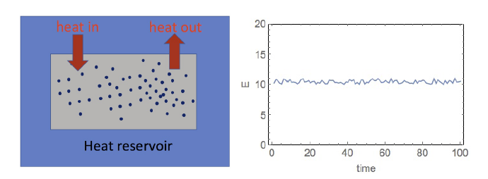
Figure 2: A canonical system in a heat bath at temperature T
Up until this point, the discussion has been purely in terms of probability theory but now we are now going to use this to model a physical system consisting of gas particles. Consider a system consisting of large number of gas particles that is in equilibrium at a fixed temperature $T$. This can be achieved by putting the system in an infinite heat bath at temperature T, and assuming that it can exchange energy, but not particles, with the heat bath (see above figure, such a system is called a canonical system in thermodynamics). The energy $E$ of the system is not fixed, but can fluctuate as shown in the right hand side of the figure. This fluctuation is due to the energy exchange with the heat bath required to maintain the temperature at a constant value T. Clearly every particle does not have the same energy level as a result of the heat exchange and since we can’t track each and every particle, all we can do is work in terms of the distribution of energies. Hence we have introduced some ‘fuzziness’ in our knowledge of the system.
Assume that the system can be in one of M states, such that in state $i$ it has energy $E_i$. Also define $p_i$ as the probability that the system is in state $i$. In the gas example with $N$ gas molecules, a state is usually defined as $(n_1,n_2,…,n_r)$ with $\sum_i n_i = N$, where $n_i$ is the number of gas molecules in a discrete quantum state $i$ with energy $e_i$. Hence the energy of the state is given by $E_i = \sum_j n_j e_j$ Another important example is a ferromagnet consisting of N atoms, such that each atom is fixed in place, but can have two spin values, oriented either up or down. In this case a state corresponds to a particular joint orientation of their individual spins, for example the state $(P,Q)$ corresponds to $P$ atoms with spins pointing up and the $Q$ atoms with spins pointing down. This system, which is called the Ising model, is analyzed in more detail in the following sections.
Recall that our ignorance or uncertainty about the system state is captured by the entropy $S$ given by
\[S = -\sum_{i=1}^M p_i \log p_i\ \ \ \ \ \ \ \ (5)\]Also the average energy of the system is given by
\[E_{av} = \sum_{i=1}^M p_i E_i\ \ \ \ \ \ \ \ (6)\]Following the modern approach to statistical mechanics, we will use the definition of entropy as the starting point in the analysis. From the mathematical point of view one can see why entropy may be an important quantity, since it is has direct connection to probabilities of the microstates $p_i$ which are critical in computing macroscopic quantities that we can measure such as $E_{av}$. But what is the physical significance of this definition for entropy? Changes in entropy can be measured in the lab, and indeed entropy was introduced into thermodynamics by Clausius well before statistical mechanics came along. For the system shown in the figure above, if its temperature is increased from $T_1$ to $T_2 > T_1$ by transferring an amount of heat equal to $Q$ from the reservoir, then the increase in its entropy is given by ${Q\over T}$ (called the Clausius formula). But according to Shannon and Boltzmann, entropy is given by equation (2), and is a measure of our lack of information about the microscopic details of a system. However this implies that the entropy is also connected with the observer, for example an observer who has a more granular view of the system may have different view of what a state is. But how can we reconcile this with the fact that changes in entropy can be objectively measured using the Clausius formula? This can be explained as follows: In the equilibrium state the number of states that result in the same macro measurement, such as temperature, is enormous. However the distribution of these states has a very sharp peak, hence even if we drill down to more granular view of the system, the states that contribute to the average value of the macro measurement are sharply concentrated around the same region in probability space.
The maximum entropy principle from the previous section tells us that that our best estimate $p_i$ that the system is in state $i$ is given by the Boltzmann distribution
\[p_i = {e^{-\beta E_i}\over Z} \ \ \ where \ \ \ Z = \sum_i e^{-\beta E_i}\]
Figure 3: Boltzmann distribution of energy levels in the Ising model with varying temperature
Plotting the Boltzmann distribution as a function of the state is a difficult proposition, since the state is multi-dimensional with thousands of dimensions in realistic models. However it can also be plotted as a function of the energy levels $E$, so instead of considering the probability of the system being in state $i$, we instead consider the probability of the system being in a state with energy $E$. For example in the above figure the Boltzmann distribution is plotted for the Ising model at four different temperatures (in blue). We can see that as the temperature increases the distribution moves towards the right, as more energetic states become more probable. Hence given the temperature we cannot say for sure what state the system is in or what energy it has, but we can estimate the probability of this happening, which is sometimes referred to as ‘blurry’ view of the system. Also the sharp peak in the distribution is evident in these curves, which implies that is a configuration is chosen at random (the red curve) then the probability that it will belong to one of the allowed configurations for a given value of $T$ is zero. If so, how would we go about obtaining the configurations in the Ising model if the system were to be simulated on a computer? There are a couple of ways for doing this, namely the Metropolis and Glauber algorithms, and these are described in a following section.
An interesting property of the Boltzmann distribution is that the statistics of macroscopic quantities of interest, such as average energy or the entropy, can be expressed as a function of $Z$ alone. Hence solving a problem in statistical mechanics reduces to calculating the $Z$ for the system, which is unfortunately quite difficult in practice. The average energy $E_{av}$ can be written as
\[E_{av} = \sum_{i=1}^N {e^{-\beta E_i}\over Z} E_i = -{\partial\log Z\over\partial\beta}\]and substituting $p_i = {e^{-\beta E_i}\over Z}$ into the definition for $S$ gives us
\[S = \beta E_{av} + \log Z = -{\beta\over Z}{\partial Z\over \partial\beta} + \log Z\]The second law of thermodynamics says that entropy of a closed system never decreases, it stays the same or increases. For the system shown in figure 2, the second law says that
\[S_{heat\ bath} + S_{gas} \ge 0\]Note that this law does not rule out a local increase in entropy, in fact this is how living systems are able to function by using the energy coming from the sun to decrease their entropy and bring order to their bodies.
But we have yet to identify the significance of the constant $\beta$. Using the above formula for $S$, it follows that
\[dS = \beta dE_{av} + E_{av} d\beta + d\log Z\]Since $Z$ is a function of $\beta$, this can be written as
\[dS = \beta dE_{av} + E_{av} d\beta + {d\log Z\ d\beta\over d\beta}\]Using the formula for $E_{av}$ the last two terms cancel off, leading to the following formula for $\beta$
\[\beta = {dS\over dE_{av}}\]But what is the significance of the derivative ${dS\over dE_{av}}$? It can be shown that if two canonical systems with energies $E_{av}(1), E_{av}(2)$ and entropies $S_1,S_2$ are connected to each other, and if initially ${dS_1\over dE_{av}(1)} > {dS_2\over dE_{av}(2)}$, then energy flows from system 2 to system 1, and in equilibrium the two derivatives are equal. This motivates the definition of temperature $T$ as the inverse of $\beta$, given by
\[{1\over T} = \beta = {\partial S\over \partial E_{av}}\]We are using the partial derivative since in the more general case S may be function of other variables such as the volume, pressure or magnetic fields for example.
Hence temperature enters statistical mechanics as the inverse of the Lagrange multiplier $\beta$ used to maximize the entropy! Note that we have derived some of the most important formulae in statistical mechanics by starting from the concept of entropy alone, which is quite amazing!
There is an useful relation between the partition functions for two or more independent systems that we will use later. If the two systems have partition functions given by $Z_1 = \sum_i e^{-\beta E_i}$ and $Z_2 = \sum_i e^{-\beta E’_i}$, then it follows from the independence assumption that the partition function for the joint system is given by
\[Z = \sum_i\sum_j e^{-\beta (E_i + E'_j)}\]which can also be written as the product of the original partition functions as follows
\[Z = \sum_i e^{-\beta E_i} \sum_j e^{-\beta E'_j} = Z_1 Z_2\]These are the classic formulae of statistical mechanics and have been known since the time of Boltzmann in the latter part of the 19th century. They represent a remarkable advance in our knowledge of the world, since they connect a quantity $Z$ which is a function of invisible microscopic properties of the system, with quantities such as $E_{ev}, T$ and $S$ that are macroscopic quantities that we can measure with our instruments. Remember that when these formulae were discovered atomic theory was still a controversial topic among physicists, in fact Boltzmann was at the receiving end of a lot of scorn since he based statistical mechanics on an unproven hypothesis. The discoveries of the 20th century validated his thinking, and in fact statistical mechanics served as a prototype for some of the great theories that were discovered, including quantum mechanics (by way of Planck and his theory of black body radiation) and quantum field theory. Late in the 20th century Hawking and others showed that even black holes possess macroscopic thermodynamic properties such as temperature and entropy, the cause for which remains un-explained.
If this had been the usual description of statistical mechanics, then at this point I would have introduced the model for an ideal gas, and then apply the formulae that we just derived to compute its average energy and entropy etc. But we are going to take a slightly different tack and focus on the Ising model for ferromagnetism instead. This system is less complex than the ideal gas, since the atoms are fixed in place rather than zipping around in space, but at the same time it enables us introduce the concept of interaction between atoms in a simpler way than for the case of a gas. In particular coupling between atoms leads to phase transitions which can be demonstrated in the Ising model without getting into very complex analysis.
Free Energy
There is another macro thermodynamic quantity that we will need later, and that is the Helmholtz free energy $F$ defined as
\[F = E_{av} - TS\]This quantity is called free energy since it is the portion of system energy that can be used to do useful work, the portion $TS$ due to entropy is pure disorder which cannot be used to do work. From the formula $S = \beta E_{av} + \log Z$ for entropy, it is easy to see that
\[F = -T\log Z\]From this equation you can start to see why $F$ might be an important quantity in statistical mechanics. We saw earlier that the partition function $Z$ plays a vital role as the connector between microscopic properties of a system and its macroscopic behavior. The equation above is essentially saying that $F$ and $Z$ are the same thing. It can be re-written as
\[e^{-\beta F} = \sum_i e^{-\beta E_i}\]which shows that $F$ is a macro distillation of all the microscopic energy interactions $E_i$ within the system.
There is another important use of the free energy, which is as a way to identify the thermal equilibrium state for the system. From the second law of thermodynamics we know that equilibrium is characterized by the maximization of entropy, but note that this is the entropy of the system plus that of its surroundings, which is not that straightforward to characterize. It turns out that thermal equilibrium can also be characterized as the state at which the free energy of a system is at a minimum (without any reference to its surroundings). In order to see this consider a system that starts at some temperature $T$ and also ends at the same temperature, but in the process draws an amount of heat equal to $Q$ from the heat bath. From the conservation of energy it follows that $\Delta E_{system} = Q$ Also the change in entropy for the heat bath is $\Delta S_{bath} = -{Q\over T}$. From the second law since $\Delta S_{bath} + \Delta S_{system} \ge 0$ it follows that $\Delta S_{systam} \ge {Q\over T}$. Thus
\[\Delta F_{system} = \Delta E_{system} - T\Delta S_{system} \le Q - T{Q\over T} = 0\]so that
\[\Delta F_{system} \le 0\]Hence for a system that only interacts with its surroundings through the exchange of heat, the free energy never increases, instead it decreases until it reaches a minimum when thermal equilibrium is reached. This implies that in a canonical system kept at constant temperature, thermal equilibrium is the state of minimum Helmholtz free energy. This criteria is very powerful since it depends on the just the system, and is independent of the surroundings. In order to use it, we need a way to calculate the free energy for a system that is not in equilibrium, we will tackle this in a later section.
When scientists say that the energy of a system is minimized in equilibrium, they are referring to the free energy, since the total energy as a whole is conserved. As a result of these advantages, the analysis of thermodynamic systems is often based on the computation of their free energy, and this is true of the systems we will encounter in this article.
Models for Magnetism
Certain atoms possess a magnetic moment, which we denote as $\mu$, due to the intrinsic spin of their outer-valance electrons. When an external magnetic field with intensity $H$ is applied, then the energy $e$ of one of these atoms is given by
\[e = -\sigma\mu H\]where the spin $\sigma = +1$ if the magnetic moment of the spin aligns with the external field, and $\sigma = -1$ otherwise.
The system we shall consider is the same as shown in figure 2, except that instead of a gas we have a $N$ atoms that are fixed in place, and can be in one of two states, with spin $+1$ or $-1$. But we still have the thermal heat bath at temperature $T$ that transfers heat energy into the system and thus causes the spin values to become dis-ordered.
We will analyze two types of magnetic materials:
- In paramagnetic materials, the individual spins are decoupled from one another. As a result the material only exhibits magnetic properties in the presence of an external field,
- In ferromagnetic materials on the other hand, individual spins are coupled with those of their neighbors, as a result of which the material remans magnetized even in the absence of the external field.
The first model for magnetic materials was proposed by Lenz in the early 1920s. He gave the problem of analyzing the model to his PhD student Ising, who was able to solve the problem for the case when the spins are arranged in $d = 1$ dimension, by using the tools of statistical mechanics. The case $d = 2$ doesn’t have a simple exact solution, and it was not solved until the 1940s by the Norwegian scientist Lars Onsager, and the case $d\ge 3$ is still unsolved. However using approximations it can be shown that models with $d\ge 2$ exhibit phase transitions, which is defined as a sudden change in the properties of a material when the temperature or one of the physical variables is reduced (or increased) beyond a certain threshold.
Phase transition is the most interesting property in thermodynamics and the Ising model is simplest system that exhibits this behavior. As a result it has become an extremely important model, and all manners of systems have been analyzed using variations of this model. It was later found out that the mathematics of Ising models and that of quantum field theory are the same, which led to a lot of cross fertilization between the two fields. In addition to Lenz and Ising, the names most associated with this model are the Russian physicists Landau and Ginzburg and Americans Wilson and Kadanoff.
Model for Paramagnetism
We will modify the notation slightly and write
\[e = -J\sigma\]for the energy of a single atom, where $\sigma$ is the same as before and $J=\mu H$ is called the coupling constant.
The partition function for a single spin at temperature $T = {1\over\beta}$, in the presence of a magnetic field can be expressed in terms of an hyperbolic function, as
\[Z = e^{\beta J} + e^{-\beta J} = 2 \cosh(\beta J)\]Now consider a system with $N$ spins, the partition function for this system is given by
\[Z = \sum_{all\ [\sigma]\ configs} e^{-J\beta\sum_i \sigma_i}\]where the sum is over all possible spin configurations. The computation of this sum can be simplified by noting that since the system is paramagnetic, the spins are independent. It follows that the partition function for a collection of N spins is given by the product of the individual partition functions
\[Z = 2^N\ \cosh^N(\beta J)\]so that $\log Z = N\log 2 + N\log[\cosh(\beta J)]$. It follows that the average energy $E_{av}$ is given by
\[E_{av} = -{\partial\log Z\over\partial\beta} = - NJ\ \tanh(\beta J)\]The average energy density on a per spin basis $e_{av}$ at temperature $T$ is given by
\[e_{av} = {E_{av}\over N} = -J\ \tanh(\beta J)\]If the thermal average of the spin on a per atom basis is $\sigma_{av}$ then since $e_{av} = -J\sigma_{av}$, it follows that
\[\sigma_{av} = \tanh(\beta J)\]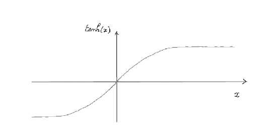
Figure 4: Average spin $\sigma_{av}$ as a function of $\beta = {1\over T}$
A graph of the $\tanh$ function is shown above. As a result of thermal energy, each spin is constantly flipping back and forth, and as a result the average spin lines between $-1$ and $+1$. Since we are considering positive temperatures only, we will focus on the half plane $\beta > 0$.
- At very low temperatures $\beta\rightarrow\infty$, and as a result the average spin $\sigma_{av} = 1$ and the average energy is minimized at $e_{av} = -J$. Hence at low temperatures the influence of the external magnetic field overcomes the random thermal fluctuations and as a result each spin becomes perfectly aligned with the external field, and this is lowest energy configuration.
- Conversely at high temperatures $\beta\rightarrow 0$ and as as result the average spin goes to zero, and so does the average energy. This implies that at high temperatures the thermal fluctuations dominate the ordering effect of the external field which results in the spins being randomly aligned in the up or down direction.
As the temperature is reduced, the spins start to gradually align with the external field, but note that there is no phase change, i.e., a sudden shift from non-alignment to alignment, it happens gradually. On the other hand, there is a phase change if the external magnetic field is switched from $+B$ to $-B$. This causes the average spin to flip to $\sigma_{av} = -\tanh(\beta J)$ (even though the average energy remains the same). This is a sudden change in the average spin, and is referred to as a phase transition of type 1.
Ising Model in One Dimension
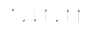
Figure 5: One dimensional Ising model
We come to our first model for an interacting particle system that incorporates interactions between neighboring atoms and the one dimensional case is discussed in this section (see the figure above). The energy for a given configuration of spins is written as
\[E = -J\sum_i \sigma_i\sigma _{i+1}\]We still have the heat bath at some temperature $T$, but unlike the previous case, there is no external magnetic field present. Each of the terms in this expression in minimized when $\sigma_i = \sigma_{i+1}$, i.e., the spins are aligned together, either with $\sigma_i = \sigma_{i+1} = 1$ or $\sigma_i = \sigma_{i+1} = -1$. This implies that there are two configurations with the minimum energy value, which correspond to all the spins pointing up or all the spins pointing down. The partition function for this system is given by
\[Z = \sum_{all\ [\sigma]\ configs} e^{-J\beta\sum_i \sigma_i\sigma _{i+1}}\]This sum has to be evaluated over all possible spin configurations, which makes it a non-trivial problem. The analysis can be simplified by defining a set of variables $\mu_i$ which is the product of neighboring spins, i.e.,
\[\mu_i = \sigma_i\sigma _{i+1},\ \ i = 1,2,...,N-1\]Note that $\mu_i$ is defined on per connection basis, rather than on a per atom basis. With this definition the partition function $Z$ becomes
\[Z = Z_1 + Z_2\]where $Z_1$ is the partition function for the case when the first spin is $+1$, and $Z_2$ for the case when the first spin is $-1$ (note that specification of the first spin, in combination with the sequence $\mu_i, 1 = 1,2,..,N-1$ allows us to recover all the remaining spins $\sigma_2,…\sigma_N$). Both $Z_1$ and $Z_2$ are equal and are given by
\[Z_1 = Z_2 = \sum_{all\ [\mu]\ configs} e^{-J\beta\sum_i \mu_i}\]But this is exactly the same partition function as for the case analyzed in the previous section, i.e., when there are $N-1$ spins in a magnetic field and there is no interaction between neighboring spins. Leveraging the solution we obtained for that case, it follows that
\[Z_1 = Z_2 = 2^{N-1}\cosh^{N-1}(\beta J)\]so that
\[Z = 2^N\cosh^{N-1}(\beta J)\]It follows that the average $\mu_{av}$ is given by
\[\mu_{av} = (\sigma_i\sigma_{i+1})_{av} = \tanh(\beta J)\]As expected, the correlation between the spins of neighboring atoms goes to zero as temperature increases, but what about low temperatures? This equation tells us that the average of the connection values $\mu_{av}$ goes to one, but from this can we conclude that the all atoms have transitioned to the up for down spin configuration? We cannot, since even if most of the spins are at $\sigma_i = 1$, there can be islands of atoms with $\sigma_i = -1$, and this is consistent with having an overall average $\mu_{av}$ of 1. Indeed it can be shown that the correlation between spins separated by $n$ positions is given by
\[(\sigma_i\sigma_{i+n})_{corr} = \tanh^{n-1}(\beta J)\]This implies that even at very low temperatures, for example for $\beta = 0.9999$, we can still make $n$ large enough so the the correlation goes to zero. From this we can conclude that there is no phase transition in the 1-D Ising model for non-zero temperature values, i.e., it does not exhibit the phenomenon of spontaneous magnetization in the absence of an external magnetic field.
Ising Model for Two or more Dimensions: Phase Transitions
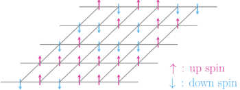
Figure 6: The Ising model in two dimensions
Spontaneous magnetization happens in a system when the spin state of even a single atom propagates through the material and re-orients all the spins. We just saw that in one dimension this does not happen, since the correlation between spins fades the further away we get, irrespective of the temperature. One way of understanding this is by noting that the spin at a particular atom in the 1D case has at most two other spins which directly influence it, i.e., those of its immediate neighbors. However for $d=2$, each atom has four neighbors, and as a result if the majority of their spins are aligned in a certain direction, then it influences the target atom to align in the same direction. Hence the presence of multiple neighbors acts as a kind of error correction when determining the spin value.
Unfortunately the exact analysis of Ising models for $d\ge 2$ is extremely difficult. However there exists a simple approximation method, called mean field analysis or MFA, that preserves important properties such as phase transitions and we will describe that next.
The energy level for a single spin $\sigma$ with nearest neighbors $\sigma_1,…,\sigma_{nn}$ is given by
\[e = -J\sigma\sum_{i=1}^{nn}\sigma_i\]The total energy for a configuration of N spins in $d$ dimensions is given by
\[E = -J\sum_{i=1}^N\sum_{j=1}^{nn(i)} \sigma_i \sigma_j\]where $nn(i)$ is the set of nearest neighbors for spin $i$. Expressing the spins in terms of their fluctuations $\delta\sigma_i = (\sigma_i - m_i)$ from their average value $m_i = (\sigma_i)_{av}$,
\[E = -j\sum_i\sum_j(m_i + \delta\sigma_i)(m_j + \delta\sigma_j)\]Expanding this expression and ignoring the product of the fluctuations $\delta\sigma_i\delta\sigma_j$ assuming it is neglegible, we get
\[E = -J\sum_i\sum_j(m_i m_j + m_i\delta_j + m_j\delta \sigma_i)\]According to the mean field approximation $m_i = m_j = m$, i.e., the mean value value of the spins is the same everywhere. This leads to
\[E = -J\sum_i\sum_j(m^2 + m(\sigma_j - m) + m(\sigma_i - m))\]From translational invariance of the spins it follows that
\[E = -J\sum_i\sum_j(2m\sigma_i - m^2)\]Note that $\sum_i\sum_j = {1\over 2}\sum_i\sum_{j\in nn(i)}$ where the ${1\over 2}$ factor avoids double counting pairs of sites and $nn(i)$ is the number of nearest neighbors of $i$. Since there is no dependence on $j$ in the summation, the inner sum is simply $\sum_{j\in nn(i)} = 2d$, where $2d$ is the number of neighbors for any atom, and $d$ is the number of dimensions. This leads to
\[\sum_i\sum_j \rightarrow d\sum_{i=1}^N\]The expression for energy simplifies to
\[E = {NdJm^2} - 2dJm\sum_i\sigma_i\]But this is simply the total energy level for a configuration of $N$ independent or paramagnetic atoms in the presence of a magnetic field with intensity $2dJm$. Leveraging the solution for this model from two sections ago, it follows that the partition function is given by
\[Z = e^{-\beta NdJm^2} 2^N\cosh^N(2dJ\beta m)\]and the average energy for the system is given by
\[E_{av} = -{\partial\log Z\over{\partial\beta}} = -2NdJm\ \tanh(2dJ\beta m)\]From this it follows that the average spin for the system is given by
\[\sigma_{av} = \tanh(2dJ\beta m)\]But in equilibrium the average spin should be equal to the mean field value, i.e., $\sigma_{av} = m$. Hence the following equation should be satisfied in thermal equilibrium
\[m = \tanh(2dJ\beta m)\]Making the substitution $y = 2dJ\beta m$, this equation can be written as
\[{y\over{2dJ\beta}} = \tanh\ y\]which can also be written as
\[{yT\over{2dJ}} = \tanh\ y\]The solution $y$ to this equation corresponds to the intersection of the line $z_1 = {yT\over{2dJ}}$ with the function $z_2 = \tanh\ y$,
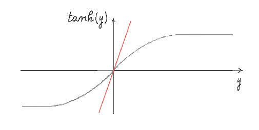
Figure 7: $z_1 = {yT\over{2dJ}}$ and $z_2 = \tanh\ y$ when $T > 2dJ$
These two functions are plotted above for the case when the temperature $T$ is very high. In this case the line $z_1$ only intersects $z_2$ at $y=0$ which corresponds to $m=0$, i.e., there is no preferred orientation for the spins. This is due to the fact that the high temperature introduces random thermal fluctuations that overcome the ordering tendency due to the mutual interactions.
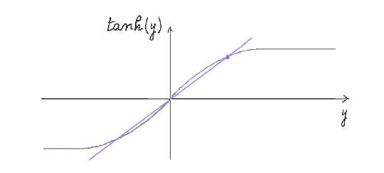
Figure 8: $\tanh\ y$ and ${yT\over{2dJ}}$ when $T < 2dJ$
However as $T$ is reduced the interaction energy due to $J$ gradually overcomes the thermal energy, and a non-zero fraction of spins become aligned on the average. This can be deduced from the above figure, since ultimately the straight line does intersect the $\tanh$ curve as $T$ is reduced, and there is a critical temperature $T_c = 2dJ$ at which the slope of the line is one, which is the same as the slope of $\tanh$ at the origin. Any decrease in $T$ beyond this point causes the two curves to intersect. When this happens there exist two other non-zero values for m, say $m’$ and $-m’$, and this corresponds to magnetization of the material. The amount of magnetization gradually increases until at very low temperatures it approaches $m = +1$ or $-1$.
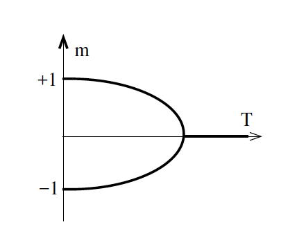
Figure 9: Variation of mean field $m$ with $T$
Since the straight line intersects the $\tanh$ curve at three places, there are three possible solutions at average spins $0$, $m’$ and $-m’$, the question arises: which one does the system choose?
- If the system starts from a low temperature state $T<T_c$ at which $m$ is non-zero and gradually increase temperature, then the magnetization initially decreases and then abruptly switches off when the temperature becomes greater than $T_c$. This would be the case if we gradually heat a ferromagnet, and is called the Curie Effect. This kind of phase transition in which there is an initial gradual decrease in the magnetization as temperature increases, followed by an abrupt change to zero beyond the critical temperature, is referred to as a second order phase transition, and is illustrated in figure 9.
- If the system starts from a state of random spins $m=0$ at $T > T_c$, what happens when the temperature is gradually reduced and crosses $T_c$? The system now has two options since there are two possible paths it can take, either $+m$ or $-m$, which one does it take? The answer is, neither. It stays in the $m=0$ state until something causes it to change state, and that something is the presence of an external magnetic field. The solution $m = 0$ is unstable if $T<T_c$, and the system can tip into the state $m\gt 0$ or $m\lt 0$ very easily, as shown next.
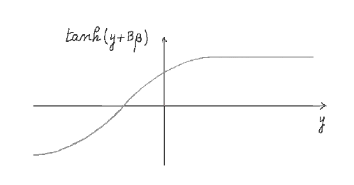
Figure 10: Graph of $\tanh(y + B\beta)$
In the presence of an external magnetic field with intensity $B$, the energy for the system is given by
\[E = -J\sum_i\sum_j \sigma_i \sigma_j - B\sum_i\sigma_i\]The first term is due to interaction with neighboring atoms, while the second term is due to the external field. Carrying out the same calculations as above, it can be shown that the $Z$ and $E_{av}$ are given by
\[Z = e^{-\beta NdJm^2} 2^N\cosh^N(2dJm\beta + B\beta)\]and
\[E_{av} = -2NdJm\ \tanh(2dJm\beta + B\beta)\]Using the same logic as before it follows that in equilibrium the mean field for the system is given by the solution to the equation
\[m = \tanh(2dJm\beta + B\beta)\]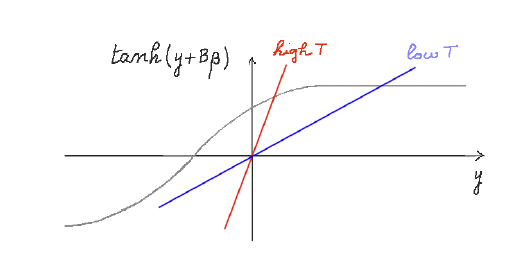
Figure 11: Graphic solution to ${Ty\over{2dJ}} = \tanh(y + B\beta)$
The solution lies at the intersection of the curves $z_1 = {yT\over{2dJ}}$ and $z_2 = \tanh(y + B\beta)$, and is plotted in the above figure. The $\tanh$ function has now shifted to the left if $B>0$, and as a result there is only one solution $m’ > 0$ to the equation, i.e., in the presence of the external magnetic field the other two solutions go away (except for the case when $\beta=0$). This means that if we were to initialize the system at $T < T_c$ with $B=0$, then we saw earlier there are three possible values for $m$, i.e. $m = 0$ or $m=m’$ or $m=-m’$. However if we switch on even a tiny amount of external magnetic field $B$, then it instantaneously causes the system to shift to $m=m’$ since the other two solutions are no longer allowed due to the shift of the $\tanh$ curve to the left. This is a phase change, and happens in ferromagnetic materials. Unlike for paramagnetic materials, the system stays in the magnetized state even after the external field is switched off. If the external field were pointing in the opposite direction, then it would have caused the system to flip to $m=-m’$.
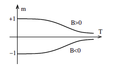
Figure 12: Variation of $m$ with $T$ in the presence of an external magnetic field $B$
The variation of $m$ with $T$ for both $B>0$ and $B<0$ is shown above, and we can see that there is no phase transition as the temperature is varied. However a phase transition does occur when the field $B$ is flipped from positive to negative or vice versa, and it causes an instantaneous change in the sign of $m$. This is an example of a first order phase transition since there is a sudden change in the phase.

Figure 13: Variation of the State Space and Magnetization of the Ising Model with Temperature
The discussion of the Ising model and phase transitions so far has been rather abstract since it has been based on a study of the equations of statistical mechanics. In order to get a more intuitive feel for changes in the system as the temperature is varied, consider the figure above. Recall that for model with $N$ atoms there are $2^{N}$ possible spin configurations. The colored ovals in the figure represent portions of the state space that are accessible at various temperatures.
- The blue area in the main oval represents part of the state space that can be accessed when $T>T_c$ and the magnetization $m=0$. This is mostly made up of states in which there are an equal number of up and down spins, but because of thermal fluctuations it also contains configurations with an imbalance in spins.
- As the temperature is reduced to a level $T_1 < T_c$, the allowed system configurations become smaller, and are represented by the light blue area in the next smallest oval. These configurations are characterized by a net magnetization $m_1$, which means more spins on the average point up than down. Note that there are two such light blue areas representing the fact that the system configuration has split up into two distinct phases.
- If the temperature is further reduced to $T_2 < T_1$, then the allowed configuration space further shrinks as shown by the orange area in the innermost oval, and furthermore the net magnetization $m_2$ increases beyond $m_1$
- In the limit as $T=0$, he ovals shrink to a single point, i.e., the configuration $(+1,…,+1)$ or $(-1,…,-1)$, since all the spins are now fully aligned with each other. Furthermore the net magnetization achieves its maximum value $m=1$ or $m=-1$, depending upon the phase.
Simulating Spin Systems
Back in the early 1950s, in the very first days of electronic computers, a group of physicists who had worked together in the Manhattan Project, got together and figured out how to simulate a system of interacting particles which are subject to thermodynamic randomness. Initially their algorithm was used to analyze neutron interactions in a nuclear reactor, and later it was applied to spin systems such as the Ising model. This group was led by Harry Metropolis, and it is by his name that the resulting algorithm is generally known. The mathematical technique that was used is called Markov Chain Monte Carlo of MCMC, and that is an alternative name for this technique.
The Metropolis algorithm is based on building a Markov Chain whose stationary distribution $\pi(\sigma_1,…,\sigma_N)$ coincides with that of the Boltzmann distribution, i.e.,
\[\pi(\sigma_1,...,\sigma_N) = {1\over Z} e^{-\beta E(\sigma_1,...,\sigma_N)}\]It works as follows:
- Start with some spin configuration $\Sigma = (\sigma_1,…,\sigma_N)$ and note that energy of this configuration is given by $E(\Sigma)$.
- Propose a move to a new trial configuration $\Sigma’$ by flipping the spin at site $i$ chosen at random, and compute its energy $E(\Sigma’)$.
- Set the spin at site $i$ according to the following rule: (1) If the move to $\Sigma’$ causes the energy to go down i.e., $E(\Sigma’)-E(\Sigma) <0$ then the move is accepted with probability $1$. (2) On the other hand if the move causes the energy to go up, then the move can still be accepted with probability $\exp^{-\beta(E(\Sigma’)-E(\Sigma))}$ and this probability decreases exponentially as $\Delta(\Sigma’,\Sigma) = E(\Sigma’) - E(\Sigma)$ increases.
The probabilistic aspect of the algorithm is implemented by using the following rule: If $\exp^{-\beta(E(\Sigma’)-E(\Sigma))} > RAND(0,1)$ where $RAND(0,1)$ is sampled over the uniform distribution $U(0,1)$, then accept the new configuration $\Sigma’$, otherwise leave the old configuration $\Sigma$.
This algorithm simulates the random spin of atoms in thermal contact with a heat bath at temperature $T$. After many steps of the algorithm, the system evolves into a Boltzmann distribution. If the system is simulated at $T>T_c$ then the thermal energy will cause it to wander among spin configurations centered at $m=0$ with no net magnetization. If $T<T_c$ then the thermal energy will still cause disordering among the spins, but a fraction of the spins will tend to get aligned in the same direction on the average, causing $m>0$.
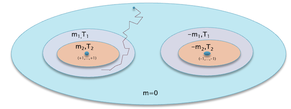
Figure 14: Example sample path in the state space while running the Metropolis algorithm
The above figure shown an example of a sample path through the state space when the algorithm is initialized at a state which is away from the equilibrium given the temperature. Assume that the model is at temperature $T_1<T_c$, while the initial state belongs to the phase $m=0$ which implies the system is not in equilibrium. The algorithm wanders randomly in the $m=0$ state space initially, and ultimately approaches the light blue ring which corresponds to equilibrium states for $T=T_1$, and once it is there is continues to wander around within the ring such that various other states occur according to the Boltzmann distribution.
Another algorithm to simulate the Ising model was discovered by Roy Glauber in the early 1960s, and works as follows:
- Start with some spin configuration $\Sigma = (\sigma_1,…,\sigma_N)$ and note that energy of this configuration is given by $E(\Sigma)$.
- Propose a move to a new trial configuration $\Sigma’$ by flipping the spin at site $i$ chosen at random, and compute its energy $E(\Sigma’)$.
- Flip the spin at site $i$ with the probability $p(\Delta E)$ given by
The Glauber rule implies that:
- As $T\rightarrow\infty$, then $p={1\over 2}$, i.e., a spin is flipped with probability half, irrespective of the change $\Delta E$ in energy.
- If $T\rightarrow 0$, then $p=1$ if $\Delta E <0$ and $p=0$ is $\Delta E > 0$. In this case it becomes a deterministic rule which says that flip with probability 1 if change in energy is negative. For intermediate values of $T$ it assumes a sigmoid shape as shown below.
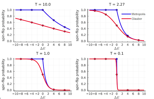
Figure 15: Comparison between the Metropolis (blue) and Glauber (red) spin flipping probabilities at various temperatures
When run long enough, both the Metropolis and Glauber algorithms lead to the Boltzmann distribution in equilibrium, however their non-equilibrium behavior is slightly different. The above figure plots the spin flipping probability for the two algorithms at various temperatures. The curves differ most at the highest temperatures, and they become almost indistinguishable at the lowest temperatures, where both curves approximate a step function.
The Landau Theory for Phase Transitions
There is an alternative approach to studying phase transitions, and this was discovered by Lev Landau around 1940, and is based on the computation of the free energy F for a system. This method significantly expanded the range of systems that could be analyzed using the methods of statistical mechanics and is now the de facto technique used. It allows us to go beyond the assumption made by mean field analysis, by allowing the magnetic field to actually vary as a function of position, thus resulting in a generalization of statistical mechanics called statistical field theory. Free energy based methods also serve as a starting point for ways in which statistical mechanics methods were first applied to the design of spin glass models, as discussed in the following sections.
The Case B = 0
Recall that the free energy $F_{therm}$ for a system in thermal equilibrium at temperature $T$ was defined as
\[F_{therm} = E_{av} - TS = -T\log Z\]I am going to generalize the definition of free energy to non-equilibrium states, which is why I have added the subscript therm to the formula. For a d-dimensional Ising Model, Z was derived in the previous section for the case $B=0$ using the mean field approximation, and is given by
\[Z = e^{-\beta NdJm^2} 2^N\cosh^N(2dJm_{eq}\beta)\]where equilibrium mean field value $m_{eq}$ satisfies the equation
\[m_{eq} = \tanh(2dJm_{eq}\beta)\]so that
\[F_{therm} = -NdJm_{eq}^2 - {N\over\beta}\log(\cosh(2dJm_{eq}\beta))\]Landau pointed out that this function can be defined even for the case when the system is not in equilibrium, thus resulting in the free energy $F(m)$ as a function of $m$, given by
\[F(m) = -NdJm^2 - NT\log(\cosh(2dJm\beta))\]From the second law of thermodynamics we know that equilibrium occurs at the minimum value of $F(m)$. Solving ${\partial F(m)\over{\partial m}} = 0$ leads to $m_{eq} = \tanh(2dJm_{eq}\beta)$. which agrees with our earlier calculations. In Landau’s theory, $m$ is called the order parameter since $m>0$ implies some degree of order which is visible at the macro level (since a larger fraction of the spins are pointing in the same direction), while if $m=0$ the spins are on the average randomized.
The next step is to understand the behavior of $F(m)$ as a function of $m$. In order to do this, we first express it as a polynomial in $m$. This is facilitated by using polynomial expansions for
\[\cosh x \approx 1 + {1\over 2}x^2 + {1\over 4!}x^4 +...\ \ \ and\ \ \ \log (1+x) \approx x - {x^2\over 2} + ...\]Substituting these in the expression for $F(m)$ we obtain
\[F(m) = -NT\log 2 + [NJd(1-2dJ\beta)]m^2 + ({2N\beta^3 J^4 d^4\over 3})m^4 + ...\]Note that $F(m)$ is symmetric with respect to $m$. Ignoring higher order terms, the derivative with respect to $m$ is given by
\[{\partial F(m)\over{\partial m}} = 2mNJd(1-2dJ\beta) + {8m^3 N\beta^3 J^4 d^4\over 3}\]It follows that $F(m)$ has a single minima at $m = 0$ if $T > 2dj$. On the other hand if $T < 2dj$ there are 2 minima, at
\[m = \pm \sqrt{ {3(2dJ\beta - 1)\over{4(dJ\beta)^3}} }\]as well as another stationary point at $m=0$. Recall the $T = 2dJ$ was identified as the critical temperature $T_c$ for ferromagnetic phase transition in the earlier analysis.
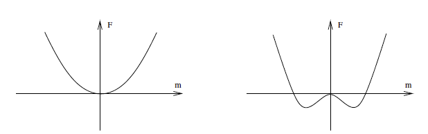
Figure 16: Free Energy $F(m)$ as a function of $m$, for $T > 2dJ$ and $T < 2dJ$
$F(m)$ is plotted in figure 10, and it clearly shows the effect of varying $T$ on its shape and provides an alternative explanation of how phase changes come about:
- When $T > T_c$ then there is only a single minima in the free energy plot at $m_{eq}=0$ and this corresponds to the non-magnetized phase.
- When $T < T_c$, there are three values of $m$ at which ${\partial F(m)\over{\partial m}} = 0$, hence the system can be one of three phases: The magnetizations $m_{eq} = \pm\sqrt{ {3(2dJ\beta - 1)\over{4(dJ\beta)^3}} }$ are stable corresponding to when spins are predominantly aligned in the up or down direction and these are the two possible phases when the system is at thermal equilibrium. However the case $m=0$ is clearly not stable since even a very small external magnetic field can cause the system to transition to the other two phases, and hence is referred to as metastable.
The other thing to note is that the equilibrium value of the magnetization $m_{eq}$ changes continuously with $T$, hence it is an example of a second order phase transition. Starting from $T<T_c$, if $T$ is gradually increased, the two minima become gradually shallower i.e, $m_{eq}$ decreases, until they disappear at $T=T_c$ at which point $m_{eq}=0$..
Using the formula
\[m_{eq} = \sqrt{ {3(T_c - T)\over{4(dJ)^3\beta^2}} }\]we can see that $m_{eq}$ has a quadratic variation with $T$ in the neighborhood of the critical temperature. This was also evident in figure 6 in the previous section. Even though this behavior was arrived at in the context of the Ising model, it turns out that all second order phase transitions for $d\ge 4$ exhibit this quadratic variation irrespective of the physical material involved. For $d = 2, 3$ the exponent is not ${1\over 2}$ (this is known from experimental data), hence the Landau theory fails for $d=2,3$. The correct exponents for these cases were computed with the help of the renormalization group theory in the 1970s.
The big advance that Landau made was the identification of a phase with the minima of the free energy function. This opened the door to the analysis of systems that have much more complicated phase behavior then the Ising model such as spin glass systems.
The Case B > 0
The analysis for this case is exactly the same as for the case $B=0$, except now the starting expression for the free energy is
\[F(m) = -NdJm^2 - {N\over\beta}\log(\cosh(2dJm\beta) + B\beta)\]Once again, using the approximations for the $\cosh$ and $\log$ functions, it can be shown that
\[F(m) = -NT\log 2 + NJdm^2 - {N\over{2T}}(B + 2dJm)^2 + {N\over{24T^3}}(B + 2dJm)^4 + ...\]Note that this expression is no longer symmetric in $m$ sue to the presence of odd powers of $m$.
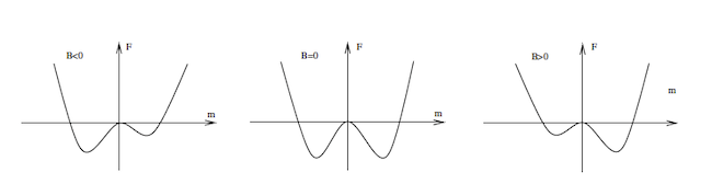
Figure 17: Free Energy $F(m)$ as a function of $m$, for $B < 0$, $B = 0$ and $B > 0$
The shape of $F(m)$ for three different values of $B$ is shown in figure 11. When $B\neq 0$, $F(m)$ exhibits an asymmetric shape as function of $m$, such that there is only a single minima (i.e., a single phase as per the Landau theory, the other phase is at a higher energy level and thus becomes metastable). This agrees with our earlier analysis that the presence of the external magnetic field removes second order temperature triggered phase transitions from the Ising model. For $B>0$ the minima that occurs for $m>0$ is deeper than that for $m<0$ (and vice versa if $B<0$). The shallower minima corresponds to a meta-stable state, and the system transitions to the more stable deeper minima by traversing the energy barrier between the two. If the sign of $B$ is flipped, then it causes an instantaneous change in the magnetization $m$ which also changes sign, and this is characteristic of first order phase transitions.
Landau’s theory clarifies some important distinctions between the minima of the energy function $E(\Sigma)$ (where $\Sigma$ is a configuration of the system), and the minima of the free energy function $F(m)$.
- It is only the free energy minima that correspond to a phase for the system. As we will see in the next section, for more complex models such as spin glasses the free energy minima are a subset of the minima for the energy function $E(\Sigma)$, i.e., there are some minima for $E(\Sigma)$ that do not correspond to a true phase for the system. These are metastable configurations and if the temperature is increased beyond zero, then the system will transition to one of the stable phases identified by the minima of $F(m)$. This has an interesting consequence for optimization problems, as we shall see in the discussion of simulated annealing.
- For $T>0$ there is more than one equilibrium configuration that realizes the $F(m)$ minima, as we saw for the Ising model. The system randomly transitions between these configurations with a probability that is given by the Boltzmann distribution. However at $T=0$, the system freezes at the maximum value of $m=1$, and at this point there is only a single configuration for the phase.
Ising Model vs Real Magnets
If we take a piece of magnetized iron and start heating it. then at a temperature above $T_c$ the magnetization will vanish, as the Ising model predicts. If we continue to increase the temperature beyond $T_c$ then the iron will become hotter, but what about the Ising model?
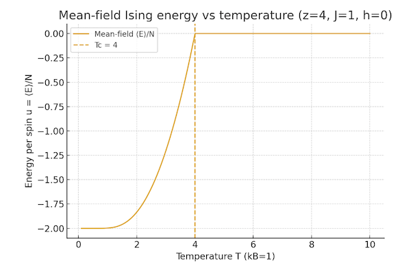
Figure 18: Plot of the average energy $E_{av}$ and magnetization of the Ising model with temperature
The heat in the iron is connected to the kinetic energy of the vibrational thermal motion of the iron atoms. However the Ising model does not incorporate vibrational degrees of freedom. In this case the increase in temperature is not associated with any further increase in the energy of the system, which can be calculated using the formula for the partition function
\[Z = e^{-\beta NdJm^2} 2^N\cosh^N(2dJm_{eq}\beta)\]so that
\[E_{av} = -{\partial\log Z\over{\partial\beta}} = - 2NdJm_{eq}\tanh(2dJm_{eq}\beta)\]This formula shows that minimum of the average energy $E_{av}$ is realized at $T=0$ and is given by $-2NdJm_{eq}$. As the temperature is increased, $E_{av}$ achieves its maximum value $E_{av}=0$ at $T=T_c$, since $m_{eq}$ goes to zero at this temperature, as shown in the above figure. Any further increase in temperature beyond $T_c$ does not lead to higher energy levels, which is somewhat counter-intuitive, but is a result of the fact that Ising model does not incorporate the vibrational degrees of freedom.
The Ising model is somewhat of a toy model in its simplicity, and leaves out a whole lot of complications in real systems. In spite of this, it does a very good job of capturing the essential aspects of magnetism, including the phenomenon of phase transitions. Why is that? This mystery was cleared up with the discovery of the theory of the renormalization group by Kadanoff and Wilson in the 1970s. They showed that natural systems are organized in hierarchies, such that the details of the lower levels of the hierarchy are completely hidden from the upper levels, and can be captured in a few a high level parameters. This is the case with the Ising model, since all that it really cares about are the spin orientations and how they interact with each other and external fields. The details of how these spins come about are not important to the model.
Spin Glass Models: Randomized Interactions
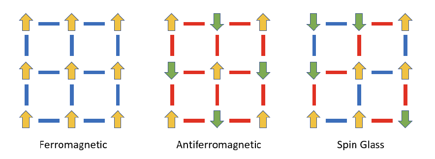
Figure 19: Spin Orientation in ferromagnetic, anti-Ferromagnetic and Spin Glass materials at $T=0$. Ferromagnetic interactions in red and anti-ferromagnetic in red.
Back in the 1950s scientists were actively investigating the properties of new materials created as a result of mixing two or more elements. This was a fruitful avenue of research and resulted in the discovery of semiconductors, that were created by adding impurities such as phosphorus to silicon. In the same spirit a group at Bell Labs created a new material by adding small quantities of ferromagnetic atoms, such as iron, to a conducting substrate, such as copper. When they studied the magnetic properties of this material as a function of temperature, they found something interesting.
- When the temperature exceeded some critical point, there was no magnetism detected, which is just as in ferromagnetic materials
- Below the critical temperature, the material become magnetic. However, after gradually increasing as the temperature was further reduced, the magnetization hit a limit at a lower level as compared to ferromagnet, and stayed at that level as the temperature was further reduced.
It seemed that the presence of the copper atoms was interfering with the tendency of iron atoms to try to align with each other as the temperature was reduced. This was a new kind of magnetic behavior not seen before, and soon physicists came up with a model for it. As shown in the above figure, all the spins of ferromagnetic materials tend to align at $T=0$, while those in anti-ferromagnetic also tend to align but in opposite directions. Spin Glasses on the other hand do not exhibit any such regularity since they contain a mixture of ferromagnetic and anti-ferromagnetic interactions. Even at low temperatures their spins can have random looking orientations as shown in the right hand side figure. In the same way that an amorphous solid like window glass doesn’t have an orderly crystal structure, a spin glass doesn’t have an orderly magnetic structure.
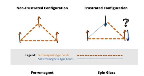
Figure 20: Illustrating Frustration
It was suggested that the random spins orientations were being caused as result of the fact that it is impossible to satisfy all the inter-node spin couplings at the same time. This results in a phenomenon called ‘frustration’ and arises whenever there exists a loop in which the product of the spins is negative. This is illustrated in the right hand side of above figure: The node in the upper vertex has a anti-ferromagnetic coupling with the node on the left, as a result of which its spin oriented downwards. But now the spin on the right side is in a conundrum. Since it has an ferromagnetic coupling with the other nodes, it doesn’t have a one best spin configuration that it can settle to in equilibrium (at $T=0$). As result it, in some cases it can settle in to an UP spin configurations and in other cases to the DOWN spin, and it chooses one of these at random. As a result there is a proliferation of metastable states i.e., a spin glass system can have many more than two phases in low temperature equilibrium, and unlike a ferromagnet, the spin configuration in a phase can look random. The thermal randomness in a ferromagnetic material gradually decreases as the temperature is reduced, and ultimately it becomes completely ordered at $T=0$. The frustration driven randomness in a spin glass on the other hand becomes “frozen” as the temperature is reduced, and it maintains the randomness even at $T=0$. We will see in the next section that there are some order parameters that are able to capture the frozen disorder in a spin glass.
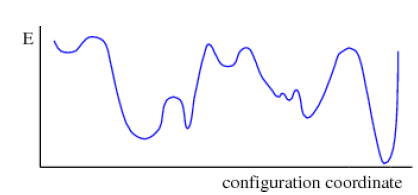
Figure 21: Energy Landscape in Spin Glasses
It was realized pretty early in the study of spin glasses that below the critical temperature their free energy landscape is quite unlike that for magnetic ferromagnetic materials. It contains multiple peaks and valleys as shown in the above figure and these seem to be quite random. From Landau theory we know that a phase corresponds to a minima of the free energy, which leads to the observation that a spin glass can have an infinite number of phases potentially. But is there an order that exists within this randomness? The discovery of such an order turned out to be a very difficult theoretical problem, and the solution did not emerge for another three decades until the mid-1980s and it won Giorgio Parisi the Nobel Prize in Physics in 2021. It also turned out that the solution to the spin glass problem had a wide range of applicability to other difficult problems which involved dis-ordered states, for example in biology, artificial neural networks and combinatorial optimization.
Edwards Anderson (EA) and Sherrington Kirkpatrick (SK) Models

Figure 22: Spin Interactions in the Sherrington Kirkpatrick Model
Samuel Edwards and Phillip Anderson were the first physicists to come up with a mathematical model for spin glasses in the mid-1970s, referred to as the EA model. In the process they introduced several new theoretical ideas that have proven to be very fruitful, but their model itself was a bit difficult to analyze. Shortly thereafter, David Sherrington and Scott Kirkpatrick introduced their eponymous model (called the SK model), which was a simplified version of the EA model, and this proved to be very influential in the subsequent years, since the model was easier to analyze also captured some of the essential aspects of spin glass behavior.
Recall that the energy function for the Ising model was given by
\[E = -J\sum_{i=1}^N\sum_{j[i]}\sigma_i\sigma_j\]This assumed that all interactions were confined to neighboring atoms (the set $j[i]$ being the neighbors of $i$), and more importantly the strength of the interaction $J$ is the same for all interactions. Sherrington and Kirkpatrick made the following modifications to this model:
- Each spin can interact with all the other spins in the lattice, and moreover interactions always happen in a pairwise fashion (see above figure) and this is called the fully connected assumption (also sometimes called the infinite range assumption).
- As in the Ising model, the spins can assume values $\pm 1$.
- The strength of the interaction $J_{ij}$ remains symmetric, but is not a constant anymore, but is a function of the two spins taking part in the interaction and can vary randomly in magnitude as well as sign.
Before the SK model, prior systems such as the Ising model sought to models systems encountered in physics, such as ferromagnets, hence all interactions were restricted to be local with neighboring spins. These models turned out to be difficult to analyze, and as we saw in the last section, physicists resorted to the mean field approximation in order to make headway. However if you think about it, the mean field approximation is a non-local assumption, since we are assuming that each spin is influenced by all the other spins in the system. Sherrington and Kirkpatrick were probably inspired by the success of the mean field model, and sought to create a spin glass model in which each spin explicitly interacts with all the other spins. Their intuition turned out to be correct, and indeed the SK model lent itself to an exact solution (though after a lot of effort). Note that the SK model does away with any spatial structure such as dimensionality since each atom is the nearest neighbor of every other atom. This assumption is a bit non-intuitive, but it turned out to be useful in applying this model to areas beyond physics, such as biology and neural networks, since in these systems the connections between nodes extends beyond nearest neighbors. The variable coupling strength $J_{ij}$ captures the fact that the interacting spins are at variable distances from each other in an actual spin glass. Under these assumptions the energy function for $N$ spins becomes
\[E = -\sum_{i=1}^N\sum_{j\lt i} J_{ij}\sigma_i\sigma_j\]For each $i$ the second sum only extends over $j$ that are less than $i$, which avoids double counting the node interactions. But what is the nature of the spin interactions $J_{ij}$? Sherrington and Kirkpatrick assumed that $J_{ij}$ can be written as
\[J_{ij} = J_{ji} = {J\over\sqrt{N}}\]where $J$ is a random variable that obeys the Standard Normal distribution, i.e.,
\[J \sim {1\over{\sqrt{2\pi}}} e^{-{x^2\over 2}}\]The scaling $\sqrt{N}$ ensures that the total energy does not blow up to infinity as $N$ increases, while the Standard Normal assumption completely randomizes all interactions. This observation lies at the heart of the SK model, i.e., the interactions can assume random values, but they follow a well defined statistical distribution.
Note that for a particular realization of the spin glass model, the random variables $J_{ij}$, are fixed or quenched, which means the $J_{ij}$ are constant on the time scale over which the spins $\sigma$ fluctuate. It would seem from this one would need all the ${N(N-1)\over{2}}$ values of the $J_{ij}$ to fully describe the SK model, which would make any analysis of the model completely intractable. Fortunately there is a property called self-averaging that comes to the rescue. Basically it says that for a single realization of the interactions $J_{ij}$, the value of macroscopic quantities, such as the free energy, can be calculated by mathematical averaging using the distribution of $J_{ij}$. This holds true for quantities that are called extensive, which means that their value scales up with the number of spins $N$. However self-averaging does not work for intensive quantities, which are defined as those whose value is independent of $N$.
We can write the free energy density for a particular realization of of $J_{ij}$ as
\[f_N(J) = -{1\over{\beta N}} \log Z\]Assume that this is well defined as the system becomes very large at $N\rightarrow\infty$, so that it converges to ${\overline f}$ defined by
\[\lim_{N\rightarrow\infty} f_N(J) = {\overline f}\]According to the self-averaging property
\[{\overline f} = -\lim_{N\rightarrow\infty}{1\over{\beta N}} E_J(\log Z) = f_{\infty}\]where the expectation $E_J$ is taken over the distribution of $J$. This property makes the analysis of the spin glass model more tractable.
The analysis of spin glass models essentially reduces to computing $E_J(\log Z)$, and this is what we will be describing in the rest of this section. Computing the partition function (or its expectation) is very hard problem in general, and the solution to some of the most intractable problems in statistical field theory and quantum field theory hinges upon this problem. There are a methods to do this that have been discovered over the years, and we are going to learn about one of these, called the replica method, in the next few sections.
Order Parameters in a Spin Glass System
We saw that the free energy for the Ising model can be described as a function of its average magnetization $m$, is this also true for spin glass systems? Define the average magnetization $m$ for the system as
\[m = \lim_{N\rightarrow\infty}{1\over N}\sum_i m_i\]where $m_i = E(\sigma_i)$ is the (thermodynamic) average of the spin at site $i$. For a ferromagnet clearly $-1\le m\le 1$ since each of the $m_i$ have a common sign. However this is not the case for spin glasses, the $m_i$’s can assume both positive and negative values. Since the random interactions $J_{ij}$ are symmetrically distributed around the origin, it follows that $m=0$ for the SK model, so that the average magnetization cannot be used as an order parameter.
So how can we characterize the magnetized phase in the SK model? If a low temperature phase exists, there must some spin configurations that are more likely to occur than others. Edwards and Anderson suggested that we use the following order parameter instead
\[q_{EA} = \lim_{N\rightarrow\infty}{1\over N}\sum_i m_i^2\]and this is called the Edwards-Anderson order parameter. For $T> T_c$, $q_{EA}=0$, since the thermodynamic average $m_i=0$. If $T<T_c$ then $m_i$ can assume both positive and negative values, $-1\le m_i\le 1$ as in the Ising model. As a result $0\le q_{EA}\le 1$ for $T<T_c$. Hence spin glass models are characterized by $m = 0,\ 0\le q_{EA} \le 1$ for $T < T_c$.
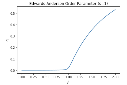
Figure 23: Variation of the Edwards Anderson Order Parameter with temperature
The above figure shows the variation of $q_{EA}$ with the inverse temperature in the SK model for the case $T_c=1$. As shown $q_{EA}$ goes to one in the limit as $T\rightarrow 0$,
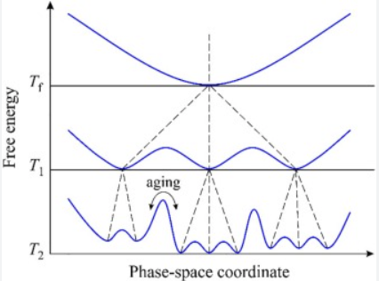
Figure 24: Free energy landscape at different temperatures
These definitions were further refined in subsequent years, with the introduction of the concept of a “pure state”, but in order to do so we first have to clarify what a state is in this context. Lets assume that the disorder $J_{ij}$ in the system is fixed with a given realization of the random interactions. The characteristic feature of a spin glass phase is the existence of very many free energy valleys which are separated by very high energy barriers (as $N\rightarrow\infty$). As shown in the top part of the above figure, when $T>T_c$ there exists only a single free energy valley, and the ergodicity of the system is not broken (i.e.. the system is capable of visiting every possible spin configuration given enough time). At temperatures $T<T_c$, in the limit as $N\rightarrow\infty$ there is ergodicity breaking, as a result of which the system in equilibrium explores only a sub-portion of the state space. Just below $T_c$ the space of spin configurations is divided into many valleys separated by infinite barriers of free energy, as shown in the middle part of the figure. Inside each of these valleys, the thermal average of a spin at each site $m^{\alpha}_i$ becomes non-zero, where $\alpha$ denotes the valley. In the literature these free energy valleys are also referred to as pure states of the system, and in this case the Boltzmann distribution becomes de-generate (or splits into sub-components). The Edwards-Anderson order parameter for pure state $\alpha$ is given by
\[q^\alpha_{EA} = {1\over N}\sum_i (m^\alpha_i)^2\]The free energy $F_\alpha$ of a pure state is given by
\[e^{-\beta F_\alpha} = \sum_{[\sigma^\alpha_i]} e^{-\beta{\sigma^\alpha_i}}\]where the sum is over the configurations that make up pure state $\alpha$. Each pure state can be assigned a statistical weight $P_{\alpha}$ given by
\[P_{\alpha} = {e^{-\beta F_{\alpha}}\over{\sum_{\gamma}e^{-\beta F_{\gamma}}}}\]Using this distribution, the average of any observable $O$ can be written as
\[E(O) = \sum_{\alpha} P_{\alpha} E(O_{\alpha})\]In the Ising model there are only two pure states, since no more than two phases (or valleys) appear as the temperature is reduced. However that is not the case for the SK spin glass model, which is characterized by a continuous series of symmetry breaking as the temperature is reduced. The lower part of the figure shows that at a temperature $T_2$ which is just below the temperature $T_1$ in the middle part, each of the three phases in the middle part have broken into multiple new phases, and this fragmentation continues all the way to $T=0$.
It was soon realized that $q^\alpha_{EA}$ was not a sufficient order parameter to characterize the system, since it is restricted to a single valley and does not give any information about the relationship between valleys in the state space. The parameter $q_{\alpha\beta}$ defined by
\[q_{\alpha\beta} = {1\over N}\sum_i m^\alpha_i m^\beta_i\]called the overlap was introduced as a measure of the extent by which two pure states are close to each other. The inverse of $q_{\alpha\beta}$ describes a metric which is like the distance between two pure states. The pure state overlap is an important parameter since we will see shortly that it serves as the order parameter for the free energy function in the SK model. Note that $\vert q_{\alpha\beta}\vert \le 1$ and in particular the self overlap is given by
\[q_{\alpha\alpha} = {1\over N}\sum_i ( m^\alpha_i )^2\]which is the same as the Edwards Anderson parameter $q_{EA}$ defined earlier. Since
\[m^\alpha_i \approx {1\over{C_\alpha}}\sum_{\alpha=1}^{C_{\alpha}} \sigma^\alpha_i\]where $C_\alpha$ is the number of configurations associated with the pure state $\alpha$, it follows that $0\le q_{\alpha\alpha}\le 1$. Note that the value of $q_{\alpha\alpha}$ grows as the number of pure states increases, since there are fewer and fewer configurations in each valley, and in the limit $q_{\alpha\alpha} =1$ at $T=0$ since there in only a single configuration associated with the pure state. On the other hand, as the temperature increases, more configurations participate in the pure state and as a result the self-overlap becomes less than one.
We also define the probability distribution of the overlap between two pure states for a given realization of the disorder $J_{ij}$, given by
\[P^J(q) = \sum_{\alpha\beta} P_{\alpha} P_{\beta} \delta(q - q^{\alpha\beta})\]If we average over $J$, then this results in ${\overline P}(q)=E_J(P^J(q))$ which can be used to characterize the spin glass model (note that it is a function of the distribution of the interactions $J_{ij}$). This distribution gives us information about the structure of the pure states and how they relate to each other, and hence a focus of the analysis of spin glass models has been to derive an expression for it.

Figure 25: The overlap distribution function $P(q)$ for a spin glass (top) and a ferromagnet (bottom)
In the Ising model there exists one pure state when $T>T_c$ (with $m_i = 0$), and two pure states when $T<T_c$, lets call them $+$ and $-$, with $m^+_i = m > 0$ and $m^-_i = -m < 0$ with equal probability. The overlaps are given by
\[q_{++} = m^2,\ \ \ q_{--} = m^2,\ \ \ q_{+-} = q_{-+} = -m^2\]Thus at high $T$, $P(q) = \delta(q)$ and the system is said to exhibit replica symmetry. For low $T$ on the other hand the spin configurations separate out into two non-overlapping pure states, with overlap distribution given by:
\[P(q) = {1\over 2}[\delta(q+m^2)+\delta(q-m^2)]\]as shown in the bottom part of the above figure. Note that in general the number of peaks of $P(q)$ is not equal to the number of pure states, but to the number of possible values taken by the overlap.
This figure also shows the contrast between the overlap distributions in the SK model vs the Ising model (note that in both cases, unlike what is shown in the figure, the maximum value of the overlap is less than 1, unless $T=0$). The upper figure shows the overlap distribution in the SK model at some temperature $T$ between zero and $T_c$, and we can see that there are a large number of possible overlaps, which implies the existence of a large number of pure states or phases. In fact in the SK model the number of phases becomes infinite as $T\rightarrow 0$ (called continuous symmetry breaking) as a result of which the overlap distribution $P(q)$ becomes a continuous function, and it is this function that serves as the order parameter for these systems. In effect the overlap distribution $P(q)$ turned out to be long sought after regularity in the random patterns of spin glass phases, and it took the best physicists in the world more than 20 years to discover it. Hence the spin glass phase configurations are random, even at $T=0$, but their overlaps follow a well defined law that can be computed. The curve tells us that the configurations in different spin glass pure states all overlap with each other, but there some pur states that are closer in overlap than others.
But how did scientists arrive at this highly non-intuitive notion of a continuous symmetry breaking? This was done through another highly non-intuitive mathematical trick called the replica method, and this is the subject of the next section.
The Replica Method
So how do we go about analyzing the SK spin glass model and compute its free energy function? Using the Landau theory for phase transitions, we start with the free energy density function $f_N(J)$ for $N$ spins for a particular realization of the interaction strength $J_{ij}$, given by
\[f_N(J) = -{1\over{\beta N}} \log{\sum_{[\sigma]}e^{-\beta H_N(J,\sigma)}} = -{1\over{\beta N}}\log Z_N(J)\]where the summation is over all possible configurations of the spins, and it has a limit as $N\rightarrow\infty$ given by
\[{\overline f} = \lim_{N\uparrow\infty}{\overline f}_N\]Since $f_N(J)$ is a self averaging quantity, it follows that that ${\overline f}$ is also obtained by averaging over the coupling distribution $J$ so that
\[{\overline f}_N = \sum_{J} P[J] f_N(J) = -{1\over \beta N}E_J(\log Z_N(J))\]where $E_J$ is the expectation over the distribution of $J$ and
\[{\overline f} = \lim_{N\uparrow\infty}{\overline f}_N\]Computing ${\overline f}_N$ is an extremely difficult exercise due to the complexity in evaluating $E_J(\log Z_N(J))$. In the 1960s a way to solve similar problems arose in the context of Quantum Field Theory, and is known as the replica method. It is based on the well known identity
\[\lim_{n\rightarrow 0} {Z^n - 1\over n} = \lim_{n\rightarrow 0}{e^{n\log Z} - 1\over n} = \lim_{n\rightarrow 0}{n\log Z + {1\over 2!}(n\log Z)^2 +...\over n} = \log Z\]Thus
\[E_J(\log Z_N) = \lim_{n\rightarrow 0} {E_J(Z^n_N) - 1\over n} = \lim_{n\rightarrow 0} {\log E_J(Z^n_N)\over n}\]where $Z^n_N$ is system consisting of $n$ independent replicas of the original system. Hence we have effectively replaced the computation of $E_J(\log Z_N)$ by that of $E_J(Z_N^n)$, which is much easier to carry out.
With the random interactions frozen at $J_{ij}$, consider $n$ independent replicas of the system. Replicas have the same couplings $J_{ij}$, but evolve independently, so that they can end up with different spin configurations. The overlap function $Q_{ab}$ between two replicas is defined by
\[Q_{ab} = {1\over N} \sum_{i=1}^N E(\sigma_i^a \sigma_i^b)\]where the expectation is with respect to the Boltzmann distribution. The free energy density for this system of replicas is given by
\[f_n(N,J) = -{1\over{\beta N}} \log Z_N^n\]Since the replicas are independent, the partition function $Z_J^n$ is given by the product
\[Z_N^n = \prod_{a=1}^n \sum_{[\sigma^a]} e^{\beta\sum_{a=1}^n\sum_{i\lt j} J_{ij}\sigma^a_i\sigma^a_j}\]where each of the summations $\sum_{[\sigma^a]}$ is over all possible configurations of the spins in a replica labeled by $a$. We are interested in computing $f_n(N,J)$ as $n\rightarrow 0$ and $N\rightarrow\infty$. We will do this by using self-averaging property, and accordingly lets define a function $f’_N(n)$ given by
\[f'_N(n) = -{1\over{\beta Nn}} \log E_J(Z_N^n)\]where
\[E_J(Z_N^n) = \sum_J p(J) Z_N^n\]Averaging over $J$ results in $n$ replicas, but they are no longer independent. Indeed they are correlated since their spins are constrained by the fact that they all follow the common interaction law given by $J$. Taking the limit $n\rightarrow 0$ and using the replica formula, it follows that
\[\lim_{n\rightarrow 0} f'_N(n) = -{1\over{\beta N}}\lim_{n\rightarrow 0}{E_J(Z_N^n) - 1\over n} = -{1\over{\beta N}}E_J(\log Z_N) = {\overline f_N}\]Taking this limit assumes that $E_J(Z^n_N)$ continues to be well defined even when the number of replicas $n$ is not an integer, which is an example of analytical continuation in mathematics.
After some manipulations, that involve the use of the Hubbard-Stratonovich transform, it can be shown that
\[E_J(Z_N^n) = \prod_{a\lt b}^n \int dQ_{ab} \exp^{-\beta nN g_n(Q_{ab})}\]where $Q_{ab}$ is the overlap function between replicas that was introduced earlier, and
\[g_n(Q_{ab}) = -{\beta\over 4} + {\beta\over 2n}\sum_{a\lt b}^n Q_{ab}^2 - {1\over{\beta n}}\log[\sum_{[\sigma_a]}\exp^{ \beta^2 \sum_{a\lt b}^n Q_{ab}\sigma_a\sigma_b }]\]where the summation $\sum_{[\sigma_a]}$ is over all possible spin configurations. Taking the limit $N\rightarrow\infty$, this expression can be evaluated by the saddle point approximation method, which leads to
\[E_J(Z_J^n)\approx \exp^{-\beta nN g_n(Q_{sp})}\] \[\approx 1 - \beta nN g_n(Q_{sp})\]where $Q_{sp}$ is evaluated at the value of $Q_{ab}$ which achieves its saddle point, i.e., at ${\partial g_n\over{\partial Q_{ab}}} = 0$. It follows that
\[f'_N(n) = -{1\over{\beta N}}{E_J(Z_N^n) - 1\over n} = -{1\over{\beta Nn}}( 1 - \beta nN g_n(Q_{sp}) - 1) = g_n(Q_{sp})\]In the final step
\[{\overline f} = \lim_{n\rightarrow 0} g_n(Q_{sp})\]So how do we get hold of the values of the matrix $Q_{sp}$ at the saddle point? The way scientists have proceeded is by making educated guesses (called ansatz) which depend on a finite number of parameters, and then computing these parameters by using the saddle point equations.
The Replica Symmetric Solution
The simplest structure for $Q_{ab}$ is known as the replica symmetric or RS solution. In this case the overlap $Q_{ab}$ between any two replicas is the same, i.e., $Q_{ab} = q_0$ for $a\ne b$ and $Q_{aa} = 1$ along the diagonal. Substituting this back into the equation for $g_n(Q_{ab})$ and taking the limit as $n\rightarrow 0$ so that $g(q) = \lim_{n\rightarrow 0} g_n(q)$, it can be shown that the saddle point for $g(q)$ occurs at $q=0$ if $T>T_c$. If $T<T_c$ then a solution with $q>0$ does exist, however this solution suffers from the issue that the resulting entropy $S$ is less than zero, which means that the solution is not correct.
Replica Symmetry Breaking (RSB)
The correct structure for the matrix $Q_{sp}$, that was proposed by Parisi, is a matrix with an iterative block structure in which the matrix elements $Q_{ab}$ depends on both $a$ and $b$.
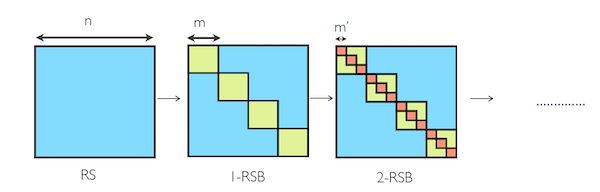
Figure 26: Illustration of replica symmetry, 1-RSB and 2-RSB, from left to right
The first two iteration of replica symmetry breaking (RSB) is shown in the above figure.
- The leftmost figure shows the case when the replica symmetry is unbroken in the high temperature case, in which all elements of the matrix are zero.
- The middle figure shows the simplest case of replica symmetry breaking, called 1-RSB. The $Q_{ab}$ matrix is parametrized by a diagonal value of $q_d$, and two off-diagonal values that can either be $q_1$ if the two replicas belong to the same inner block of size $m\times m$, or $q_0$ if one of the replicas fall outside the innermost block.
- This procedure can be iteratively repeated within each of the inner blocks, and after $k$ iterations it leads to k step RSB or k-RSB. An example of 2-RSB is shown in the rightmost figure with corresponding parameters $q_0, q_1$ and $q_2$.
- The complete solution is obtained in the limit $k\rightarrow\infty$, in which case the elements of the matrix become a function $q(x), 0\le x\le 1$.
To summarize, we have obtained a solution for the free energy ${\overline f}$ as a function of the elements of the matrix $Q_{ab}$, which can be regarded as an order parameter and this order parameter is the overlap between configurations belonging to different replicas. But what is the interpretation of this solution in terms of the spin glass model? We answer this in the next sub-section.
Connection between Replica Symmetry Breaking and the Spin Glass Model
We defined the probability distribution of the overlap between two pure states ${\overline P}(q)$ a couple of sections ago, and it turns out that this function can be expressed in terms of the replica matrix as follows:
\[{\overline P}(q) = \lim_{n\rightarrow 0}{2\over{n(n-1)}} \sum_{a\gt b} \delta(q - q_{ab})\]This equation is saying that the probability that two pure states of the system have overlap $q$ is equal to the fraction of elements of the overlap matrix $Q_{ab}$ that are equal to $q$. This means that the elements of the replica overlap matrix (after taking the limit $n\rightarrow 0$), are the physical values of the overlap between pure states, and the number of elements of $Q_{ab}$ that are equal to q is related to the probability of $q$. Hence surprisingly the matrix $Q_{ab}$ that arose a result of a mathematical trick to simplify calculations, also has a deep connection to the physics of the spin glass model.
We now apply this formula to the $Q_{ab}$ matrix that was proposed in the previous section.
The Replica Symmetric Solution
In this case $q_{ab} = q_0$ for all values of $a$ and $b$. From the above equation it follows that
\[{\overline P}(q) = \delta(q-q_0)\]This is saying that there is only one possible value $q_0$ for the overlap between pure states, and this value must be the self-overlap of the unique pure state in the system. This is typically the paramagnetic state which exists at high temperatures. Hence the replica symmetric solution is only valid if there is a single pure state, which is the case at high temperatures.
The 1-RSB Solution
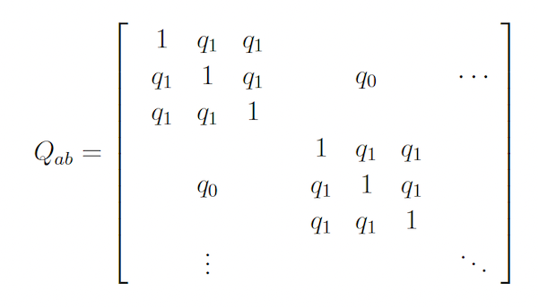
Figure 27: The $Q_{ab}$ matrix for first order RSB
The $Q_{ab}$ matrix for the 1-RSB solution as per the Parisi ansatz is shown above. This solution splits up the replicas in groups of size $m$ such that overlap between replicas within a group is $q_1$, and between groups is $q_0$ ($m=3$ in the figure). The overlap distribution is given by
\[{\overline P}(q) = {m-1\over{n-1}}\delta(q-q_1) + {n-m\over{n-1}}\delta(q-q_0) \ \ \ with\ \ \ 1\le m\le n\]We now have to take the limit as $n\rightarrow 0$ to complete the replica solution. This does not make much sense mathematically since we are effectively reducing the size of the overlap matrix to zero. However it can be argued that this limit can be taken in a mathematically formal manner (similar to raising a number to a fractional power, such $x^{1\over 2}$ for example). In this limit $m$ must also be promoted to a real number, rather than an integer. This results in
\[{\overline P}(q) = (1-m)\delta(q-q_1) + m\delta(q-q_0)\ \ \ 0 \le m \le 1\]so that $m$ is interpreted as a probability in the limit as $n\rightarrow 0$. In this equation $q_1$ can be interpreted as the self overlap and $q_0$ as the cross overlap between two distinct pure states. So now we need to determine the parameters $m, q_0, q_1$ to complete the 1-RSB solution. This can be done by substituting these numbers back in the expression for $g_n(Q_{sp})$, and then finding the values of $m, q_0$ and $q_1$ at the saddle point for this expression.
There is a class of spin glass models called p-spin spherical model or PSM discussed in the next section, in which the 1-RSB solution is exact, i.e., there is no further breaking of the replica symmetry as the temperature is reduced. However this is not the case for the SK model, and in this case the symmetry keeps breaking ad-infintum as the temperature is reduced. This results in the sequences
\[q_0 \lt q_1 \lt q_2 \lt ....\] \[m_1 \gt m_2 \gt m_3 \gt ...\]and in the limit at $k\rightarrow \infty$, it results in a continuous overlap distribution function ${\overline P}(q)$.
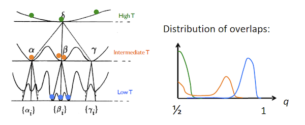
Figure 28: Illustration of replica symmetry breaking
The left hand side of the above figure shows the changes in the free energy landscape as the temperature lowered, and the distribution of the overlaps is shown on the right:
- At high temperatures there is only a single pure state and the energy landscape is fairly flat, so that individual configurations are widely spread out and have a low degree of overlap. This is illustrated by the green curve on the right which shows that the overlaps have a single peak at the zero overlap value.
- As the temperature is reduced below the critical value, we see the formation of multiple pure states and there is split of the of overlap distribution into a bi-modal shape (orange curve). Configurations can be in the same pure state in which case they have a high overlap value $q_1$, or they can be in different pure states, in which vase the overlap tends to be smaller at $q_0$.
- An even further reduction in the temperature causes more replica symmetry breaking, as a result of which we now see that each of the pure states from the second stage have further split into multiple pure states lying within the energy valley formed in stage 2. Furthermore the overlap distribution has developed a peak near 1, which implies that at low temperatures each pure state converges to its single configuration with a low degree of overlap with the other configurations (blue curve). In this situation the self overlap becomes equal to 1, while the cross overlap between states is zero. This process is completely probabilistic, so the system may end up in a different configuration every time it is gradually frozen.
Hence there are two cases in which there is low cross overlap between configurations, but the reasons are different for each: (1) In the high temperature case the cross overlap is low due to thermal activity, since each spin is flipping back and forth due to the heat energy, (2) At $T=0$ once again the cross overlap is low, but the reason is different. The spins have converged to random looking configurations, but the randomness is due to the randomness in the interaction strengths. The spins themselves are no longer flipping randomly between states since $T=0$.
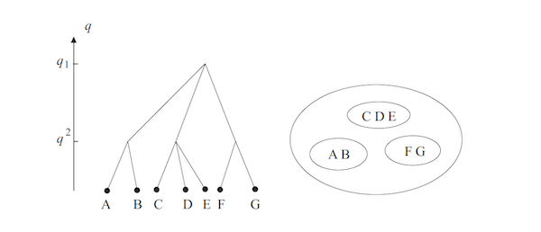
Figure 29: Tree like and nested structure in replica symmetry breaking
Another way to visualize replica symmetry breaking is shown in the above figure. At high temperatures we have single pure state, as shown by the large oval (which can be thought to be the space of all configurations) on the right and the top node in the tree. When the temperature dips below $T_c$ the state splits into three pure states as shown by the three smaller ovals which are now restricted to a smaller subset of configurations. A further reduction in temperature causes these 3 pure states to split into 6 pure states, each with a even smaller set of possible configurations. The overlap function $q_{\alpha\beta}$ depends on how far the pure states $\alpha$ and $\beta$ are from each other in the tree structure. For example A and B are closer to each other, and further away from the other states C,D,E,F and G.
Counting the Number of Pure States
In the analysis in the last section we showed the existence of multiple overlap values with replica symmetry breaking, but this only gives indirect confirmation about the existence of multiple pure states. For example in 1-RSB there are just two overlap values, but potentially a large number of pure states that have these overlaps. Note that each pure state has a well defined local magnetization at site $i$ given by $m^\alpha_i = E(\sigma^\alpha_i)$, where the expectation is restricted to a single pure state $\alpha$. A pure state is determined by its vector of magnetizations $(m^\alpha_1,…,m^\alpha_N)$. It turns out that it is possible to define a function $f_{TAP}(m_1,…,m_N)$, called the Thouless-Anderson-Palmer (TAP) free energy, whose local minima coincide with the pure states of the system. It is given by
\[m_i = \tanh[\beta\sum_j J_{ij}m_j - \beta^2 \sum_j J_{ij}^2 (1-m_j^2)m_i]\]The equivalent equation for the minima in the case of the Ising model was given by $m=\tanh(\beta m)$. The TAP equations correspond to the stationary points for the following free energy
\[f_{TAP} = -{1\over 2}\sum_{i\ne j} J_{ij}m_i m_j - \sum_i h_i m_i - {\beta\over 4}\sum_{i\ne j}J_{ij}^2 (1-m_i^2) (1-m_j^2) + {T\over 2}\sum_i[{1+m_i\over 2}\log{1+m_i\over 2} + {1-m_i\over 2}\log{1-m_i\over 2}]\]Note that the free energy is a function of the magnetizations $m_i$ and not the individual spins $\sigma_i$, hence its minima do not necessarily coincide with the energy minima, i.e., the minima of the Hamiltonian $H(\sigma_1,…,\sigma_N)$. This is result of the fact that at temperatures greater than zero, multiple energy minima may be separated by barriers that are small enough so that they belong to the same pure state.
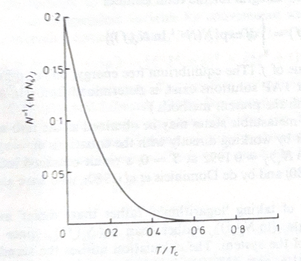
Figure 30: Logarithm of the total number of TAP solutions, divided by N, as a function of temperature
Bray and Moore proposed that the density of solutions to the TAP equation $N_s(f_{TAP})$, should be counted as a function of the free energy $f_{TAP}$, and they showed that it varies as
\[N_s(f_{TAP}) \sim \exp^{\alpha N}\]The quantity $\alpha$ is plotted in the figure above.
For the case $T=0$ the TAP equation reduces to $m_i = sign(\sum_j J_{ij}m_j)$ and by working directly with this equation it can be shown that
\[{1\over N}E_J (\log N_s) = 0.1992\]The p-Spin Spherical Spin Glass Model (PSM)
The SK model was the first spin glass model to be fully analyzed and understood. However its behavior, including the continuous symmetry breaking for $T<T_c$ is quite complex, and it would be nice to have another spin glass model with simpler phase properties. One such model that has become popular in recent years is the p-spin Spherical Spin Glass Model (or PSM) (see Castellani and Cavagna). This model can be used to analyze certain types of neural networks and thus provides a way in which the loss function in these networks can be studied using the tools from spin glass theory.
In the PSM model, p-spins interact with one another and the Hamiltonian of the energy levels for a given configuration of spins is given by
\[H_p = -\sum_{i_1>...>i_P} J_{i_1,...,i_p}\sigma_{i_1}...\sigma_{i_p},\ \ \ p\ge 3\]Thus we have multiple spins being able to interact with another at the same time. The sum is extended over all groups of $p$ spins, not only the nearest neighbors, so there is no spatial structure. Hence just as for the SK model, we can consider the PSM to be a type of mean field model, but with a greater degree of coupling between spins. Note that unlike the SK model, the spins in PSM are now real continuous variables. In order to keep the energy finite, the following constraint, called the spherical constraint, is imposed
\[\sum_{i} \sigma_i^2 = N\]Under this constraint the self-overlap of each configuration is one (which is also true for the SK model, but remember that in PSM model the $\sigma_i$’s are no longer $\pm 1$).
Any group of $p$ spins have a random interaction strength given by $J_{i_1,…,i_p}$, which is distributed according to the Normal distribution given by
\[p(J_{i_1,...,i_p}) = {N^{p-1}\over{\pi p!}} e^{[ -{(J_{i_1,...,i_p})^2 {N^{p-1}\over{ J^2 p!}}}]},\ \ \ p\ge 3 \]This system can be analyzed using the replica method just as for the SK model. For $T>T_c$ there is no net magnetization and this corresponds to the replica symmetric case. For $T<T_c$ there is first order RSB, which results in the overlap distribution
\[{\overline P(q)} = (1 - m)\delta(q-q_1) + m\delta(q-q_0)\ \ \ with \ \ \ 0\le q_0 \le q_1 \le 1\ \ \ and\ \ \ 0\le m\le 1 \]where $q_1$ and $q_0$ are the self overlap and cross overlap parameters for pure states of the system. The parameters $m, q_0, q_1$ can be determined by solving the saddle point equations for the free energy of the system, and this results in $q_0 = 0$, i.e., the cross overlap between different pure states is zero. The values of $m$ and $q_1$ are determined by solving additional equations (which I am going to leave out, the interested reader can refer to Section 3.5 of Castellani and Cavagna). It has been shown that this 1RSB solution is exact for the PSM model, i.e., there is no further symmetry breaking as the temperature is further reduced below $T_c$.
There exists an analogue to the TAP equation in the PSM model, which can be used to count the number of pure states when $T<T_c$. When this analysis is carried out, it results in the surprising discovery: The solutions to the TAP equation are given by $m_i = \sqrt{q}\sigma_i$, where the $\sigma_i$ are the minima of the energy function and $q$ is the self overlap. These are obtained by solving the equations
\[{\partial H(\sigma)\over{\partial\sigma_i}} = 0,\ \ \ \sum_i\sigma_i^2 = N\] \[{1\over N} {p\over{2}} q^{ {p\over{2}}-1 } H(\sigma) + {\partial R\over{\partial q}} = 0\]where
\[R = 1-{1\over{2\beta}}\log(1-q) - {\beta\over 4}[(p-1)q^p - pq^{p-1}]\]Note that the solutions $\sigma_i$ to the first equation do not depend on the temperature, however the value of the self overlap $q$ does. Hence in a PSM there is a 1-1 mapping between the minima of the Hamiltonian and the minima of the free energy. At $T=0$ the two coincide, but as the temperature is increased, thermal fluctuations cause the minima to occur as pure states. The PSM model is an exception to the rule that the minima of the energy function and the free energy function are not all the same, in this case they are the same!
Simulated Annealing
Kirkpatrick, Gelatt and Vechi applied the Metropolis algorithm to the problem of combinatorial optimization, and called the resulting technique simulated annealing. Combinatorial optimization is the problem of minimizing a cost function $f(x_1,x_2,…,x_N)$, and this can be likened to the energy function in statistical mechanics. If we try to find the minimum using a brute force search over the configuration space, there is a good chance that the optimization will get stuck at a local minimum, and this is the same problem that occurs when we try to find the lowest energy configuration for a spin system at $T=0$.
Kirkpatrick et.al. proposed adding a temperature variable to the optimization, which results in random thermal spin fluctuations, and then using the Metropolis algorithm to find the low energy configurations. This allows the optimization to jump out of local minima as long as $T>0$ with finite probability, since these are metastable configurations. They proposed that the optimization start at a high temperature, and then lower the temperature by slow stages, until the system “freezes” and no further changes occur. At each temperature the simulation should proceed long enough for the system to reach equilibrium.