OFDM or How the World of Ubiquitous High Speed Wireless Came To Be
Introduction
Those of you who are old enough will recall the era before 2010 when Nokia, Motorola and Blackberry dominated the market for wireless handsets. These phones had become quite proficient in handling mobile voice calls, but when it came to data, the bitrates that they provided were not quite good enough. It was possible to do some text based web surfing, but for full graphics based web pages or you tube video streaming, they were not quite up to the task. All this changed in 2011, when suddenly mobile phones suddenly became as good as desktop terminals in running even the most graphics rich web content, and streaming video became omnipresent.
So what changed? It was not due to the iPhone, since this handset had been launched a few years earlier in 2007. What changed was the cellular wireless technology, as the transition from 3G networks to 4G happened right around 2011. This article is about a key technology in 4G wireless that enabled higher data rates, called Orthogonal Frequency Division Multiplexing or OFDM. The name sounds rather formidable, but I think it is possible to explain the essence of how OFDM works even to the non-specialist with knowledge of freshman college level math, and I am going to make an attempt to do so. OFDM exists at the bottom of the communications protocol stack, also called the Physical Layer, and most people don’t even know about its existence, since most of the attention is grabbed by handsets such as the iPhone and the applications running on it. But without OFDM, high speed communications on the iPhone would not have been possible.
Before I launch into OFDM and 4G wireless, I want to briefly mention the technology that they replaced, namely 3G wireless. The latter was launched in 2001, and was the first technology that seriously tried to integrate voice AND data communications capability into the handset. Unfortunately the 3G protocol was designed in the era when voice was still based on an older technology called circuit switching, and thats what went into 3G. Data was considered to be the less important feature, hence its design was an add-on to voice. Unfortunately circuit switching is not the best way to handle data, which does better with a technology called packet switching, and this handicapped 3G phone performance. The other big issue with 3G was the Physical Layer protocol that was used, which was based on a technology called Code Division Multiple Access or CDMA. CDMA paired well with circuit switching, but it was not very well suited for data. However it had a very strong political backing, in the form of the companies Qualcomm and Ericsson which held a number of important CDMA patents. So the transition from CDMA to OFDM is also a story of how an insurgent technology, promoted by a few small start-ups, was able to overcome the powerful forces that were aligned against it.
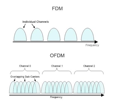
Figure: OFDM vs Regular Frequency Division Multiplexing
The basic idea behind OFDM is not that difficult to grasp, and an analogy can be made with the shift in the computer hardware industry that happened in the early 2000s. After the launch of the web in the mid 1990s, focus shifted to building more and more powerful servers that could be used for serving web pages, and for a time companies such as SUN Microsystems thrived by supplying this market. However it soon became clear that even the most powerful single machine could not keep up with the demand. Fortunately companies such as Google pioneered the concept of a datacenter made up of thousands of cheap commodity Dell type servers. By working together in parallel, these machines became capable of scaling up to serve even the most demanding workload. At the same time, this “Datacenter as Computer” architecture made the system more robust, since it could easily recover from the loss of a few of the machines at any one time, due to the redundancy that was built into the system. Hence there was a shift from single monolithic system that was expensive and prone to failure, to a distributed robust system with thousands of subsystems, which could easily scale up.
Exactly the same dynamic occurred in wireless systems. The broadband wireless technologies that came before OFDM (called single carrier QAM modulation) worked by having each transmission occupy the entire channel spectrum (see top part of above figure). Using up all the bandwidth increased the resulting bit rate to broadband speeds, and this technology is still in use for cable model systems. However for wireless transmissions, single carrier system QAM came up against a fundamental limit to how much bitrate a single channel could support, and this was first pointed out by Claude Shannon in the 1940s. Shannon showed that the ultimate capacity C in bit per second of a channel with bandwidth B Hertz, is given by the following rather simple looking formula:
\[C = B\ \log (1 + {S\over N})\]Here ${S\over N}$ is the signal to noise ratio for the channel, and this ultimately limits the data capacity of a channel if B is fixed. Wireless transmissions are subject to all kinds of channel impairments, due to the fact that they are completely exposed to the environment, which causes them to have a lower ${S\over N}$ compared to cable modem systems for example, in which all transmissions occur in a heavily shielded wired medium. The most insidious cause of lower signal to noise in single carrier QAM systems is due to a wireless specific problem called multipath self interference, and it turns out that increasing the bandwidth B makes it worse. Also increasing the power S does not help much either, since the interfering signal also becomes stronger thus causing the ${S\over N}$ ratio to decrease!
Using a single carrier QAM system for wireless transmissions is like using a single powerful CPU to run a job, and the only way to scale up single CPU systems was by making the clock speed faster and faster. This ultimately runs up against the fundamental physics of semiconductor technology, which can be considered to be a type of Shannon capacity that limits the speed of single CPUs. Computer systems got around this bottleneck by using thousands of less powerful CPUs working together to solve a problem, and as shown in the bottom part of the figure, communication engineers came up with a similar strategy.
OFDM can likened to splitting up the data stream and carrying it on hundreds of smaller pieces of spectrum, called subcarriers in the jargon. Each of these subcarriers is now carrying much less data compared to single carrier system, but since there are thousands of them, they make up for lower capacity by working in parallel, and thus are able to achieve at least an equivalent data rate in theory, and a much higher data rate in practice.
OFDM systems are much more robust in the unforgiving wireless environment. Multipath self-interference only affects a subset of OFDM sub-carriers, a phenomenon also called Frequency Selective Fading. The system can then choose not to use those subcarriers or use a more robust transmission scheme for these, while still be able to use the good parts of the spectrum. Using the Data Center analogy, if some of the computers in the Data Center are mal-functioning, the system can still keep operating albeit at a lower efficiency. Single carrier systems QAM on the other hand don’t work very well in a wireless environment, since problems that are localized in the spectrum end up affecting the entire transmission.
It would not be an exaggeration to say that today we are living in the age of OFDM! Whether you are surfing the web on your cellphone, or streaming movies on your cable modem, or connnecting to the web over WiFi at the coffee shop, it is all happening over links that use OFDM modulation. It is the base technology on which our modern connected world runs.
Historical Notes
I had some personal involvement in the transition from 3G to 4G wireless, and had a first hand view of the politics involved. I was a co-founder of a start-up called Aperto Networks that did some of the work that ultimately resulted in 4G, and for a number of years I was a member of the IEEE 802.16 Standards Committee that was working on 4G, even chairing the Medium Access Control or MAC group for a while. The MAC protocol lies on top of PHY layers such as CDMA or OFDM, and it had to completely re-designed for packet based wireless communications. But this article is not about the MAC, perhaps it will be a subject of a future article.
OFDM was invented by Robert Chang from Bell Labs in 1966, but his original proposal was too expensive to implement. The technology was proposed its current more implementable form by Weinstein and Ebert, also from Bell Labs, in 1971. Unfortunately it was a technology that was ahead of its time, and Bell Labs itself did not show any interest in commercially deploying it. It stayed in this dormant state until the 1990s, when the Internet became widespread, and broadband access to the home became a critical bottleneck. A start-up called Amati Communications applied OFDM (which they called Discrete Multitone Modulation or DMT) to solving the difficult problem of transmitting at broadband speeds over the twisted pair copper cabling that existed in all homes to support land-line voice communications. In 1993 they successfully demonstrated that they could achieve speeds of 2 mbps over twisted pair, that was much better than the 32 kbps modems that were used for data communications at the time. OFDM was subsequently adapted as the ADSL standard for sending broadband data over twisted pair and was deployed widely. Amati was acquired by Texas Instruments in 1997.
Amati also proposed OFDM for cable modems in the IEEE 802.14 Standards Group that was working in cable modem standards. I was a member of this group, it was there during 1995 that I first heard the term OFDM being mentioned, in a presentation by Amati. The Hybrid Fiber Coax of HFC plant used for cable is much more hospitable to digital transmissions compared to twisted pair, and as a result the initial cable modem standards which came from Cable Labs in 1998, and was called DOCSIS 1.0, used the less robust and simpler Single Carrier QAM modulation scheme. Ultimately cable also adopted OFDM with the DOCSIS 3.1 release of the standard, which happened in 2013. The motivation was for using OFDM in this case was not so much for a more robust channel, but for realizing higher bitrates using wide channels (wider than the standard 6 MHz used for regular cable TV), something that single carrier QAM could not do.
The standardization of OFDM in wireless communications took a two pronged path, since there were two standards bodies that were working on wireless standards at that time:
- The smaller standards body was IEEE 802, which had two committees working on wireless: The IEEE 802.11 that was working on wireless LAN, and the IEEE 802.16 that was working on a wireless MAN (or Metropolitan Area Network, which includes cellular wireless) standard. I was a member of the latter body, which started its work in 1999.
- The larger body was called 3GPP (for 3rd Generation Partnership Project), and was charted with developing standards for cellular wireless systems. Hence technologies from 2G wireless onwards, all the way to the current generation of wireless called 5G have come from this group.
3GPP was filled with a mixture of huge service providers such as AT&T or Verizon, as well as large vendors such as Ericsson and Huawei that sell equipment to them. IEEE 802.2 on the other hand was dominated by companies from the computer industry, which tended to be smaller, fast moving and more entreprenual. Consequently they were the ones that provided an opening for a new untested technology like OFDM to enter, in contrast to the more conservative 3GPP group. The first wireless standard to adopt OFDM was IEEE 802.11a for wireless LANs, and it was introduced in 1999.
The path of OFDM through the IEEE 802.16 group was more convoluted, and took longer. Initial proposals were in favor of single carrier QAM modulation, and the push for OFDM came from a tiny Israeli start-up called RunCom. Initially focus of IEEE 802.16 was on what is called Fixed Wireless (which was a competitor to cable modems or ADSL and was the focus of my start-up Aperto), but the group underwent a big change in 2004 with the entry and active participation of the chip giant Intel.
Intel wanted to position IEEE 802.16 as a competitor to the 3G wireless technology from 3GPP that was beginning to be deployed at that time. Their strategy was to use a much superior wireless technology that could support broadband data and which they could then use to compete against Qualcomm in the cellular wireless space. Intel completely upended IEEE 802.16 by establishing another standards body called WiMAX in 2005, to come up with the standard. With Intel’s backing, WiMAX decided to make a radical break in wireless modem technology, and adopted Runcom’s OFDM proposal for the physical layer. The other important piece of technology in WIMAX, i.e., the Medium Access Control protocol was heavily influenced by some of the work that Aperto had done for their proprietary system called PacketMAX, and constituted my contribution to this story.
WiMAX was adopted by some of the big equipment vendors such as Samsung and Nokia, and the service provider Sprint actually started deploying this technology in 2007 in the Washington DC area. I briefly worked for Sprint in their Herndon office at that time, and I could see the excitement in the organization about the new possibilities that WiMAX opened up. I thus got an early preview of the world of streaming video and high speed web surfing over wireless handsets, that became widely available a few years later.
There were two powerful holdouts against WiMAX, namely the chip company Qualcomm and the equipment provider Ericsson. They correctly identified WiMAX as a way in which Intel could bypass the semi-monopoly that they enjoyed in the 3G cellular space, and thus dominate the next generation of wireless technology. They also recognized the shortcoming of 3G technology in support broadband data, and consequently abandoned the next generation CDMA technology they had been developing, and made the pragmatic decision to focus 3GPP, which was working on the standards for 4G at that time, into using OFDM as well! But this was going to be the 3GPP version of OFDM, not the OFDM technology that was developed by WiMAX. Qualcomm and Ericsson had sufficient clout among the large service providers, who subsequently all threw their hat behind the Qualcomm-Ericsson version of OFDM, which came to be called LTE, for Long Term Evolution. All the other big vendors saw the writing on the wall and adopted LTE as well, and the current 4G era began with the LTE deployments by Verizon in the US, that began towards the end of 2010. WiMAX was continued to be deployed by Clearwire Wireless (which was the company to which Sprint had sold its WiMAX division), but withered away due to lack of support from the service provider community.
So much so for history, what does the future hold? An excellent overview of the ways in which 5G Wireless is attempting to improve bitrates can be found here. The rest of this article is going to get deep into OFDM technology, which involves a little bit of math, mainly the math of the Fourier Transform. But it is worth the effort.
The Fourier Transform
To get to an understanding of how OFDM works, it is necessary to know a mathematical technique called the Fourier Transform. It was first published by Joseph Fourier of France in the 1820s, and since then it has become one of the most powerful tools in the arsenal for mathematicians and engineers. The Fourier Transform is another example of the 2-Layer Principle for organizing complex data, that I written about in an earlier article called Latent Variables and Latent Spaces. The principle states that a complex system can often be represented in two ways: (1) As it exists in the real world, and thus can be measured using instruments, and (2) In an abstract mathematical space, which we can access only by performing some mathematical operations on the real world data. Moreover the two representations can be inter-changeably transformed into one another. The abstract representation Lyer 2 is often easier to manipulate and analyze, and a number of difficult problems in the real world can be solved, by first solving the problem in the abstract space. Other examples of this 2-Layer Principle from the earlier article include:
- Representing data such as images and language using Latent Variables. The mathematical transformation in this case is represented by Artificial Neural Networks. This representation lies at the heart of all the progress being made in this field.
- Representing physical phenomenona using the idea of Fields. This started with Maxwell and the Electromagnetic Field, and went on to represent matter using Quantum Fields. Also the Schrodinger Wave Function for a particle can be represented either in terms of its location x in space, or its momentum p, and these two representation $\psi(x)$ and $\psi(p)$ are Fourier Transforms of each other!
It can be argued that a great deal of scientific progress in the last 200 years has been made by exploiting the 2-Layer Principle. The Fourier Transform can be considered to be the original example of this principle, and hence it is fitting that the fundamental duality of matter in terms of waves and particles is intimately connected with it. Within the realm of communications systems, this transform can be used to represent a signal that exists in time, into an abstract representation that is instead based on the frequencies that signal occupies. It is not an exaggeration to say that almost all of the progress in communications theory in the last 100 years is based on exploiting the properties of the frequency based representation which is also called the spectrum of the signal. By using the spectral representation, we are able to manipulate time based signals in various ways, which would be impossible to do otherwise.
Before launching into the Fourier Transform, I am going to introduce a simpler version, that was also discovered by Fourier, called the Fourier Series.
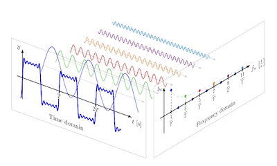
Figure 1: Decomposition of a time domain signal into its frequency domain components
The fundamental idea behind the Fourier Series is illustrated in Fig. 1, which shows a periodic time domain signal with period T (in approximate square wave shape, in the lower left of the figure). Fourier proposed that any such periodic signal can be represented as a linear combination of sine and cosine functions, also called tones, whose frequencies are integer multiples of the base frequency $f = {1\over T}$, as follows
\[x_N(t) = a_0 + \sum_{n=1}^N \left[a_n\cos{2\pi nt\over T} + b_n\sin{2\pi nt\over T}\right]\]This decomposition of a complicated function into its tones is known as the Fourier Series. Note that we make the number N of tones larger, the approximation becomes more and more exact. The transform can also be understood by thinking in terms of musical notes. Expert musicians are said to have the ability to make out individual tones in a complex piece of music, their brain is essentially carrying out the Fourier Transform!
You can see why $x(t)$ is constrained to be a periodic function with period T, since both sine and cosine are periodic with this period. In this case the Layer 2 representation for the signal $x(t)$ is the set of coefficients ${a_0, a_1, b_1, a_2, b_2, …}$. Hence we have replaced a complex time based periodic function, by an equivalent representation which consists of a bunch of numbers, which is a huge amount of simplification. Fourier’s insight was his realization that this decomposition could be done for any periodic function $x(t)$ (a few decades later Peter Dirichlet gave more rigorous conditions that $x(t)$ has to satisfy for the decomposition to work) . Fourier showed that these coefficients can be computed using the formulae:
\[a_0 = {1\over T}\int_{-{T\over 2}}^{T\over 2} x(t) dt\] \[a_n = {1\over T}\int_{-{T\over 2}}^{T\over 2} x(t)\cos{2\pi nt\over T} dt,\ for\ n\ge 1\] \[b_n = {1\over T}\int_{-{T\over 2}}^{T\over 2} x(t)\sin{2\pi nt\over T} dt,\ for\ n\ge 1\]There is an equivalent representation of the Fourier Series using complex numbers, which utilizes the Euler Formula $e^{j\theta} = \cos\theta + j\sin\theta$, and is as follows:
\[x_N(t) = \sum_{n=-N}^N c_n e^{2\pi nt\over T}\ \ \ where\ \ \ c_n = {1\over T}\int_{-{T\over 2}}^{T\over 2} x(t)e^{-2\pi nt\over T} dt\]where the new coefficient $c_n$ is now a complex number. The quantity $1\over T$ is the frequency $f$, and using this notation the equations become
\[x_N(t) = \sum_{n=-N}^N c_n\ e^{2\pi nf t}\ \ \ where\ \ \ c_n = {1\over T}\int_{-{T\over 2}}^{T\over 2} x(t)\ e^{-2\pi nf t} dt\]Since the Fourier Series can only be used for periodic signals, what about aperiodic signals that occur just once in time. This is where the Fourier Transform comes into the picture, and is given by the formulae:
\[x(t) = \int_{-\infty}^{\infty} X(f)\ e^{2\pi ft} df\] \[X(f) = \int_{-\infty}^{\infty} x(t)\ e^{-2\pi ft} dt\]Thus the Fourier Transform of an aperiodic time function $x(t)$ is a dual aperiodic function $X(f)$ that exists in the frequency space. Hence if $x(t)$ is aperiodic, its representation is no longer a discrete set of numbers, but instead becomes a function $X(f)$ that exists over a continuum of frequences! In order to provide an heuristic justification for these formulae, note that in the Fourier Series representation, two neighboring frequencies are separated by $\Delta f = {1\over T}$. We can convert a periodic $x(t)$ into an aperiodic function by making $T$ larger and larger, and in the limit as $T\rightarrow\infty$, we can see that the separation between adjacent frequencies in its Fourier Series representation goes to zero, which is a hand-wavy of saying that the frequencies now form a continuum (also the product $nf$ approaches a finite quantity, as $n$ goes to infinity and $f$ goes to zero).
The Discrete Fourier Transform
The Fourier Transform works well enough for signals that are continuous in time, but we live in a digital world, and the computers that we depend on can only process discrete numbers. In order to enable this, a continuous signal has to be discretized, before any further processing can be applied to it and furthermore the Fourier Transform has to be able to work for discrete signals. The next few figures go through the discretization process, and the resulting transform called the Discrete Fourier Transform or DFT. OFDM utilizes DFT in a critical part of its design, hence the focus on this.
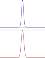
Figure: Fourier Transform (in red) for a signal (in blue)
As before, let $x(t)$ be a continuous time signal that is defined over the interval $[0,1]$ with Fourier Transform $\tilde X(f)$.
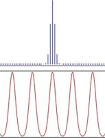
Figure: Fourier Transform (in red) for a signal that is sampled in time (in blue)
Let $x[n]$ denote samples of this signal, taken at the rate of $f_s={1\over T_s}$ samples/second, where $T_s$ is the sampling period. Furthermore assume that N samples are taken over the interval $[0,1]$, so that $N={1\over T_s}$. Thus we have
\[x[n] = x(nT_s), \ \ \ for\ \ \ 0\le n\le N-1\ \ \ and\ \ \ 0\ \ \ otherwise\]Furthermore assume that $X(f)$ is the Fourier Transform of $x[n], 0\le n\le N-1$, so that
\[X(f) = \sum_{n=0}^{N-1} x[n]\ e^{-j2\pi fn},\ \ \ 0\le f\le 1\]From this equation we can see that $X(f)$ is a periodic function. Hence discretization in the time domain causes periodicity in the frequency domain.
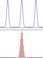
Figure: Inverse Fourier Transform (in blue) for a signal that is sampled in frequency (in red)
If, instead of discretizing the time domain signal $x(t)$, what will happen if we discretize the frequency domain signal $\tilde X(f)$? If we evaluate ${\tilde X}(f)$ only at discrete values of frequency $[0, \Delta f, 2\Delta f,…, (N-1)\Delta_f]$, where $\Delta f = {1\over N}$, and defining $X_k = {\tilde X}(k\Delta f]$, then what is its Inverse Fourier Transform? The result of this operation is shown in the above figure and as can be seen, it results in a periodic and continuous function in time.
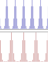
Figure: Fourier and Inverse Fourier Transforms for a signal that is sampled in both time and frequency
Finally, what would be the result if both the time domain and frequency domain functions were to be discretized as shown in the above figure? This results in the Discrete Fourier Transform, whose equations are given by:
\[X_k = \sum_{n=0}^{N-1} x[n]\ e^{-j2\pi {k\over N}n},\ \ \ for\ \ \ k=0,1,...,N-1\]This formula can be inverted to obtain
\[x[n] = {1\over N}\sum_{k=0}^{N-1} X_k\ e^{j2\pi {k\over N}n} \ \ \ for\ \ \ n=0,1,...N-1\]The last two equations constitute the Discrete Fourier Transform and the Inverse Discrete Fourier Transform respectively. Note that these transforms allow signals to be processed in the digital domain.
You may be wondering that by discretizing a continuous time signal, we may be throwing away useful information. But in fact this is not the case, as was proven by Harry Nyquist, who worked in Bell Labs in the period prior to World War 2, I will have more to say about him in the next section. This work was further extended by the legendary Claude Shannon, so the work is referred to as the Nyquist-Shannon Sampling Theorem. The theorem states that as long as we sample a signal fast enough, it is always possible to re-create the original signal from the samples. The minimum sampling rate for perfect re-construction is $2B$, where $B$ is the maximum frequency in the Fourier Transform of $x(t)$. This is an amazing result, and one can get an intuitive understanding of why is is true by examining the second figure in this section. It shows that if a continuous time signal is discretized, then its resulting Fourier Transform is just the periodic continuation of $\tilde X(f)$, where the latter was the Fourier transform of the continuous time signal $x(t)$. Hence if we were to filter out just one of these shapes, and take its Inverse Fourier Transform, then we would have recovered the original signal $x(t)$!
Designing the Best Signal: The Nyquist Pulse
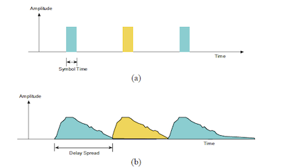
Figure: Sending Morse Code Data (a) Transmitted Data (b) Received Data
At the dawn of the Communications Age, when Samuel Morse was experimenting with ways in which he could send the Morse Code pulses across a telegraph line, he noticed that received pulses tended to get smeared out in time (see above figure), and thus interfere with neighboring pulses. In order to avoid this, he left enough of a gap between pulses, as shown in the figure. This solved his problem, but at the cost of a reduced data rate. In our own digital age, all data is in the form of 1s and 0s, and the communications engineers working in the early years of digital transmission, faced exactly the same problem, i.e., how to reliably get the bits across the channel without them interfering with each other.
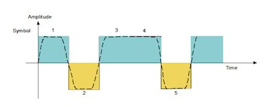
Figure: Sending the Sequence 101101 using Square Wave Pulses
Consider the back-to-back transmission of the bit sequence 101101 using Square Wave pulses of the type that Nyquist was using, as shown above.
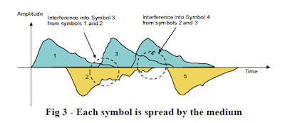
Figure: Sending the Sequence 101101 using Square Wave Pulses
This figure shows the corresponding signal at the receiver, and we can see that the bits have smeared into one another.
Harry Nyquist came up with a solution to this problem during the 1930s. His name is not that well known to the general public today, but the contributions that he made laid the foundations for both communications and control theory, and later scientists who came after him, like Claude Shannon, built upon his work. Nyquist decided to attack the problem of optimal pulse design in order to avoid inter symbol interference, and the main tool that he used for this was the Fourier Transform.
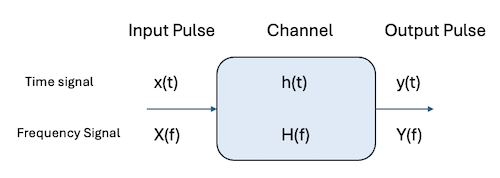
Figure: Signal Filtering due to Channel
When a pulse is sent through a channel, its shape gets distorted due to its interaction with the channel. This can be captured in the frequency space by the following equation:
\[Y(f) = H(f)X(f)\]were $H(f)$ is called the Transfer Function of the channel, while $X(f)$ and $Y(f)$ are the Inverse Fourier Transforms of the input and output pulses respectively. $H(f)$ is the inverse Fourier Transform of the impulse response of the channel $h(t)$, which is obtained by sending a very short narrow signal, approximating the Dirac Delta Function into the channel. This equation clearly captures the distorting effect of the channel on the input signal.

Figure: Adding Transmit and Receive Filters to the System
Nyquist proposed that we add two filters to the system, as shown above, namely the Input Pulse Shaping Filter and the Output Pulse Shaping Filter. The input-output response of the system is now captured by
\[Y(f) = R(f)H(f)G(f)X(f)\]The filter frequency responses $G(f)$ and $R(f)$ are under the control of the designer, and thay can be tailored so as to eliminate Inter Symbol Interference. Next Nyquist searched for for pulse shapes $Y(f)$ at the receiver that have no Inter Symbol Interference.
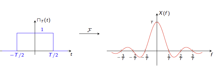
Figure: Time Domain Square Pulse and its Fourier Transform
So what kind of pulse shape should we use to avoid ISI? The Fourier Transform comes to our rescue in solving this problem. The above figure shows the Fourier Transform for a square pulse $x(t)$ in the time domain with pulse duration $T$, which we will also refer to as the Symbol Time. Its Fourier Transform results in the so called sinc function $X(f)$ in the frequency domain, given by
\[X(f) = {\sin \pi f T\over{\pi f}}\]Note that $X(f)$ is symmetric around $f=0$ and it has zeroes at the frequency values ${n\over T}$ for integer values of $n$. A pulse such the one shown is called a baseband pulse, since its Fourier Transform is centered at $f=0$. (When computing the bandwidth, or frequencies occupied by the spectum, we only consider the half plane $f\ge 0$, by this criteria the bandwidth for the pulse shown in the figure is ${1\over T})$.
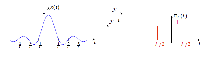
Figure: Time Domain Sinc Pulse and its Fourier Transform
Next lets invert the problem by using the sinc sunction as the input, with zeroes at ${n\over F}, n=1, 2,…$ where $F = {1\over T}$, given by
\[x(t) = {\sin {\pi F t\over{\pi t}}}\]From the prior discussion it follows that its Inverse Fourier Transform is given by a square pulse $X(f)$ in the frequency domain, as shown in the above figure. It turns out that the time domain sinc pulse is the optimum signal shape to avoid Inter Symbol Interference as discussed next.
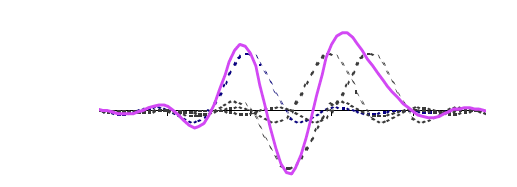
Figure: Resulting waveform in time when sending 1011 Using 4 Sinc Pulses
Note the time domain version of the sinc has zeroes at $nT$ for integer values of $n$, and this property is very useful when sending a train of pulses back to back, separated by the period $T$. The above figure shows the resulting waveform when the bit sequence 1011 iis transmitted using a stream of sinc pulses separated by time $T$. Just as in the case of square pulses, the signal for a particular pulse leaks over to other pulses, but with one big distinction: The peak of a pulse, coincides with the zeroes of all the neighboring pulses which follows from the fact that the sinc has zeroes at integer multiples of $T$! This property implies that there is no Inter Symbol Interference between neighboring sinc pulses, even when they are stacked next to each other at intervals of $T$.
Based on this observation, Nyquist proposed that the filters $G(f)$ and $R(f)$ should be designed in such a way so that the product $Y(f) = G(f)H(f)R(f)$ results in a frequency domain shape of a square pulse. This will ensure that the time domain output pulse shape $y(t)$ at the receiver would be a sinc function, with zero Inter Symbol Interference. In order to make the $G(f)$ and $R(f)$ filters realizable using circuitry, he derived a slightly modified form of the sinc pulse, known as a Raised Cosine Pulse, and these are in use for digital communications even today. The sinc function has the property that its Fourier Transform X(f) uses up the least amount of bandwidth, and a more efficient pulse shape has not been found. They are now called Nyquist Pulses in his honor.
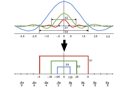
Figure 3: Effect of Sinc Pulse Width on Bandwidth
Another very important property of sinc pulses is the variation of bandwidth with the width of a pulse. As the pulse width T decreases, the bandwidth required for transmission increases, as shown in the above figure (for the case $T=1$). In general the required bandwidth for a sinc pulse of duration $T$ is ${1\over{2T}}$, i.e., one half the symbol rate. This is a very important property that tells us that as we increase the rate at which are transmitting data into the channel by decreasing $T$, the corresponding channel bandwidth needed increases at the rate of ${1\over {2T}}$.
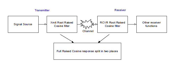
Figure: End to End Baseband Communication System
The individual filters $G(f)$ and $R(f)$ are implemented as Root Raised Cosine Filters or RRC, and these are designed such that their serial operation results in the Raised Cosine pulse shape, as shown above. Inter Symbol Interference mitigation using sinc pulses works well enough as long as the channel is reasonably good. However wireless channels exhibit something called multipath interference, which needs additional work to mitigate.
In the discussion so far we haven’t talked about how data bits actually get mapped to the signaling waveform such as the sinc pulse. Since we are sending analog waveforms over the channel, we have the freedom to modify the waveform so that instead of sending only two types of waveforms (say +sinc and -sinc which map into the bits 0 and 1), we can choose to send four types of waveforms (say +2sinc, +sinc, -sinc and -2sinc), which allows us to map 2 bits to each waveform, thus doubling the bitrate for a given symbol rate. This topic is discussed in detail in the next section.
Baseband communication systems are an important topic in their own right, and are used in sending digital data over media such as twisted pair copper loop whose frequency response is centered at zero. However, channels in wireless and cable systems are centered at higher frequencies, and thus the baseband signal has to be shifted before it can be transmitted, and this is the subject of the next section.
Designing Signals with Multiple Levels and Phases: Single Carrier QAM Modulation
Data transmission over a wireless or cable systems requires that the signal energy be confined to an assigned frequency slot in the spectrum, called a channel (for example cellular 4G communications happens over channels that are allocated in various frequency bands between 600 MHz and 2.4 GHz). How can we shift our signal from the baseband to a channel with a larger center frequency? Once again the Fourier Transform comes to the rescue, as shown in the figure below.
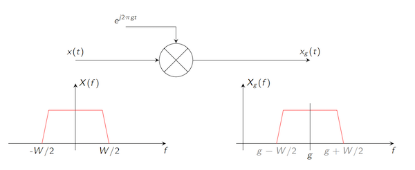
Figure: Shifting the Center Frequency of a Signal
If we take a baseband signal and multiply it by a complex exponential at frequency $g$, then the Fourier Transform tells us that the resulting signal now occupies a channel whose center frequency is precisely $g$. This can be shown using the following calculation: If $X(f)$ is the Fourier Transforms of $x(t)$, then the Fourier Transform of $x_g(t) = x(t) e^{j2\pi gt}$ is given $X(f-g)$ (see above figure). An application of the Euler Formula $e^{j\theta} = \cos\theta+j\sin\theta$ leads to the result that Fourier Transform of $x(t)\cos (2\pi f_0 t)$ is given by ${X(f-f_0)+X(f+f_0)\over 2}$. This is the property that we are looking for, i.e., the ability to shift the spectrum occupied by the baseband pulse. The resulting waveform is known as a passband pulse and the cosine function used to do the translation is called the carrier wave.
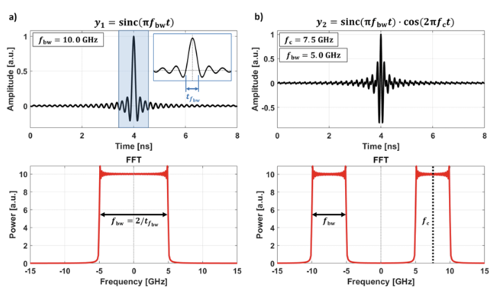
Figure: (a) A Baseband Sinc Pulse and its Fourier Transform (b) A Passband Sinc Pulse and its Fourier Transform. The baseband pulse has been shifted by 7.5 GHz.
The shift in frequency of a baseband sinc pulse from 0 GHz, as shown in column A, to 7.5 GHz, as shown in column B, is illustrated in the above figure. Note that as a result of the shift, the bandwidth occupied by the passband pulse is double that of the baseband pulse, i.e., for a sinc pulse of width $T$, the baseband bandwidth that it occupies is ${1\over{2T}}$ while its passband bandwidth usage is ${1\over T}$.
The use of the carrier wave allows us to use its parameters as another way in which sinc pulses can be differentiated. In particular we can use both the amplitude of the sinc pulse as well as the phase of the carrier wave to differentiate pulses. Hence it is now possible to define a so called constellation of passband sinc pulses, with differing amplitudes and phases, and this is called Quadrature Amplitude Modulation or QAM. One of the simplest QAM constellations uses four different signals and is called Quadrature Phase Shift Keying or QPSK, and we will describe that next.
The basic idea behind QPSK is quite simple and goes as follows: The incoming bit stream gets grouped together two bits at a time, followed by a mapping to one of four waveforms described below, for $0\le t\le T$, where $T$ is the symbol time:
- Bit pattern 00 gets mapped to the carrier wave $\sqrt{2}A\cos(2\pi f_c t + {\pi\over 4})$.
- Bit pattern 10 gets mapped to $\sqrt{2} A\cos (2\pi f_c t + {3\pi\over 4})$.
- Bit pattern 11 gets mapped to $\sqrt{2} A\cos (2\pi f_c t + {5\pi\over 4})$.
- Bit pattern 01 gets mapped to $\sqrt{2} A\cos (2\pi f_c t + {7\pi\over 4})$.
We can see that the different bit patterns are differentiated based solely on the phase of the carrier wave. This mapping can be nicely represented in the complex plane as follows:
- Bit pattern 00 gets mapped to the complex number $({1\over{\sqrt 2}}, {j\over{\sqrt 2}}) $
- Bit pattern 10 gets mapped to $(-{1\over{\sqrt 2}}, {j\over{\sqrt 2}})$
- Bit pattern 11 gets mapped to $(-{1\over{\sqrt 2}}, -{j\over{\sqrt 2}})$
- Bit pattern 01 gets mapped to $({1\over{\sqrt 2}}, -{j\over{\sqrt 2}})$
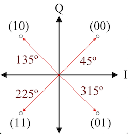
Figure: Passband Modulation using Quadrature Phase Shift Keying or QPSK
These four values numbers can be plotted on the complex plane as shown above.
Using this mapping the QPSK waveform can be written as:
\[x(t) = \sqrt{2} A [Re(a)\cos(2\pi f_c t) - Im(a)\sin(2\pi f_c t)] = Re[\sqrt{2} A a e^{2j\pi f_c t}],\ \ \ 0\le t\le T\]where the complex number $a$ takes on one of the four values from the mapping above, depending upon the bits being transmitted. The numbers $\sqrt{2} A Re(a)$ and $\sqrt{2} A Im(a)$ are also referred to as the I and Q components of the signal $x(t)$ (they stand for in-phase and quadrature phase). Using these equations, the QPSK transmitter can be implemented as shown below:
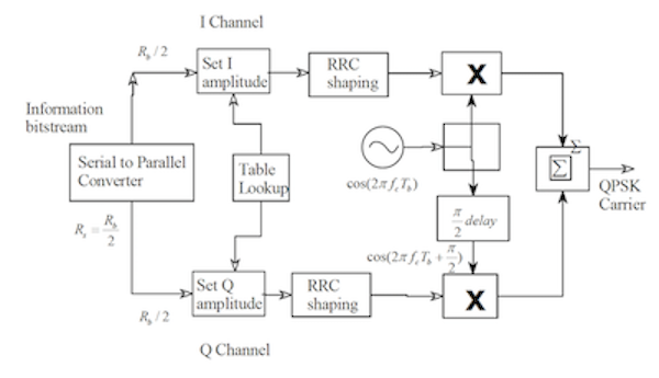
Figure: A Single Carrier based QPSK Modulator
The figure shows that the incoming bit stream on the left is first converted to consecutively occurring pairs of bits in the Serial to Parallel Converter. Since 2 bits map to a single symbol, the resulting symbol rate $R_s$ is half of the bitrate $R_b$. The table lookup mapping from bit pairs to the complex number $a$ is then used to determine the Real and Complex parts of $a$, which determine the I and Q components of signal. Next the baseband pulse for the signal is generated by using the Nyquist Root Raised Cosine (RRC) Filter in order to avoid Inter Symbol Interference, as discussed in the prior section. This is followed by multiplication of the I and Q components by the carriers $\cos(2\pi f_c t)$ and $\sin(2\pi f_c t)$ respectively, in order to shift the pulse to the center frequency $f_c$. Finally the two components are subtracted to generate the signal to be transmitted.
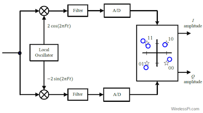
Figure: A Single Carrier based QPSK De-Modulator
A QPSK receiver is shown above. The incoming waveform is first multiplied by the carrier $f_c$ so as to shift it in frequency to the baseband and separate its I and Q components. This is followed by the receive RRC filtering, and finally sampling to recover the numbers $Re(a)$ and $Im(a)$, which are then mapped to one of the bit pairs.
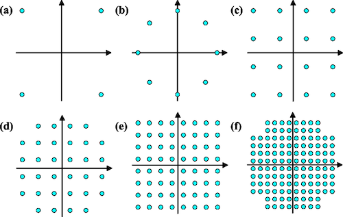
Figure: Higher Level Signal Constellation (a) QPSK (b) 8-PSK (c) 32-QAM (d) 16-QAM (e) 128-QAM
The bitrate for a single carrier system can be increased over that of QPSK by packing more bits into a single symbol. This can be done by increasing the number of possible waveforms, which can be done either by varying the phase of the carrier or its amplitude. As for QPSK, this can be conveniently illustrated on the complex plane, as shown in the above figure, which shows the I and Q components for a few higher order modulations. For example 128-QAM maps 7 bits to each symbol, so that the resulting bit rate is 3.5x that of QPSK (for the same symbol rate).
So how far can this process go, i.e., can we keep increasing the constellation size and realize greater and greater bitrates? It turns out that with more sophisticated systems it is possible to increase it by quite a bit. For example the cable modem standard DOCSIS 3 specifies that 4096-QAM is mandatory, while 8192-QAM and 16,384-QM are optional on cable modems! But ultimately, this technique runs into the Shannon Channel Capacity limit $C = B\log (1+{S\over N})$, since packing more constellation points means that they will move closer and closer to each other, and at some point the noise in the channel will make it impossible to differentiate one symbol from another. In fact DOCSIS 3.1, which is the latest iteration of the standard, now specifies that OFDM be used instead of QAM, which allows even higher bitrates by increasing the channel bandwidth $B$ without compromising on the error performance.
The Wireless Channel
In order to understand why Single Carrier Modulation QAM does not work very well over wireless, we first have to understand a few things about the nature of impairments that affect transmissions in this type of channel. There are quite a few of them, including:
- Interference from other wireless system operating the vicinity. This is less of a problem in the licensed frequency bands like LTE, but even here there could be interference from neighboring cells using the same frequency band.
- Wireless propagation related issues: As for all electromagnetic waves, the transmitted power falls off as the inverse of the square of the distance. But a bigger source of decrease in signal strength is the fact it is expected to penetrate one or more walls on the way to the receiver. Each time it does so, its power can reduce by up to two orders of magnitude.
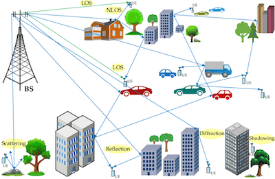
Figure: Sources of Multipath Interference
There is another more serious problem that afflicts wireless systems, that of multipath, and is illustrated in the figure above. Multipath is due to the fact that the transmissions encounter a lot of clutter on their way from a high transmit antenna, to the handset that is usually located at street level. As a result the transmitted signal bounces around from the objects in the environment, and several copies of the signal arrive at the receiver within a few microseconds of another. For example the figure shows signals arriving at the handset in a moving vehicle after bouncing off one or more buildings, other vehicles in the vicinity etc. We have all come across multipath in other type of networks, such as when occasionally we hear echoes on a long distance VoIP connection, or an on-screen visual impairment called ‘ghosts’ in an over the air TV transmission (in which multiple copies of objects appear on the screen).
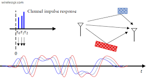
Figure: Inter-Symbol Interference due to Multipath
The superposition of multiple copies of the same signal, separated in time, at the receiver (shown in the above figure) leads to a situation where they can completely cancel each other out, called destructive interference, or they can reinforce each other, called constructive interference. The situation where the signals cancel each other is referred to as deep fade, and before the advent of OFDM, it plagued broadband wireless systems that were using single carrier QAM modulation.
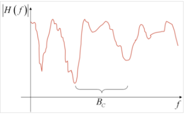
Figure: Frequency Response of a Wireless Channel
It is possible to plot the frequency response of a wireless channel, and one such plot is shown the above figure. We can see that the response amplitude is not uniform with frequency, but exhibits dips at various points in the spectrum. This is precisely due to the effect of multipath propagation.
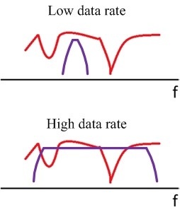
Figure: Channel Response compared to the Signal Spectrum for Narrowband (top) and Broadband Systems (bottom)
So why does multipath affect single carrier QAM systems more than previous generation of narrowband systems such as 2G or 3G. One way to understand this is by examining the channel frequency response.
- If the transmissions are of the narrowband type, then there is a good chance that their spectrum is fully contained in the flat part of the channel response, as shown in the top part of the figure, which alleviates the problem. This scenario is called Flat Fading.
- However if it is a broadband QAM signal, then its pulse width in time is much narrower and a result, its signal spectrum becomes wider, as was explained in the section of Nyquist Pulses. The wider signal spectrum spans the part of the channel spectrum with the deep fade notches, which lead to reception problems, as shown in the bottom part of the figure. This scenario is called Frequency Selective Fading.
Another problem is that the channel is dynamic, especially if the receiver is moving around, so the location of the notches in the channel response can constantly change during the duration of a single data session.
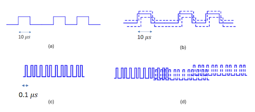
Figure: Illustration of Interference in the Time Domain for Narrowband Systems (top) and Broadband Systems (bottom)
Multipath interference can be understood more directly by examining its effect in the time domain, and this is shown in the above figure. It illustrates the case when the bit sequence 100101 is transmitted using a symbol time of 10 us in the top two figures and 0.1 us in the bottom two figures. The 10 us symbol corresponds to a narrowband transmission, and part (b) we can see two multipath signals arriving with a time offset at the receiver. The amount of multipath delay is of the order of 1-2 us, which is much less than the symbol time of 10 us. This is the case that corresponds to Flat Fading, and there are well known techniques to combat it. With the broadband signal on the other hand, since the symbol time is only 0.1 us, the 1-2 us delay spread in the multipath now affects many more symbols in the future, as shown in part (d) of the figure, and this corresponds to the case of Frequency Selective Fading. Note that with single carrier QAM modulation, the symbol time decreases as we increase its occupied bandwidth, so the frequency selective problem becomes worse at higher data speeds.
OFDM OR How Data is Sent over a Broadband Wireless Link
Is there a more robust way to transmit broadband data over a wireless channel, which does not suffer from multipath interference? It turns out there is, and it was first proposed by Robert Chang from Bells Labs in 1966, building on some earlier work by Franco and Lachs. He discovered OFDM by inverting the transmission problem in some sense, from the time to the frequency domain, by using the magic of the Fourier Transform.
Recall that Nyquist showed us that it is possible to stack up baseband pulses right next to each other in time, with their peaks separated by an interval of $T$, and still avoid Inter Symbol Interference, as long as we shape them using the sinc function, and this results in a bandwidth usage of ${1\over{2T}}$ for the signal. The only way to send data faster is by making the pulse width $T$ smaller, which results in a larger bandwidth used. But there is another way to avoid Inter Symbol Interference, as Morse discovered almost 200 years ago, which is by leaving a large gap between successive time pulses. However this technique is not compatible with broadband communications, since it leads in a big reduction in the symbol rate. But is there a way out of this conundrum?
It turns out there is! If we transmit very large symbols (in time), this allows us to leave a relatively small gap between successive symbols without losing too much capacity. But large symbols lead to smaller symbol rate if we are using single carrier QAM modulation. However what if we transmit multiple symbols in parallel at the same time? Hence each symbol will carry a smaller amount of data by itself, but in aggregate all the symbols together can carry as much data in a given interval of time as the single carrier QAM case. This is exactly what OFDM does!
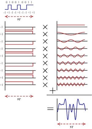
Figure: Generating an OFDM Symbol
But how can we transmit multiple symbols in parallel, without them interfering with one other? This is were genius struck, with the idea that the parallel transmissions can be made independent of each other, by multiplying them with carrier waves that are orthogonal to each other. This allows each individual symbol to be recovered at the receiver, by multiplying it with the carrier wave at the same frequency that was used for transmitting that symbol. As Fourier showed, carrier waves, which are just sine and cosine functions, can be made orthogonal to each other by making sure that their frequencies are integral multiples of each other.
The process of generating a single OFDM symbol is shown in the above figure. Let say we have to transmit the 9 bit sequence 010010011, shown in top part of the figure. If we use Single Carrier QAM modulation, then the transmission of each bit will take T seconds (assuming BPSK modulation), for a total time of 9T seconds. With OFDM, we are going to use up the entire 9T seconds to transmit a single symbol (or bit in this case), as shown in the left side of the figure. We multiply each symbol by a carrier whose frequencies are integral multiples of each other, an shown in the right hand side. We then add up all the 9 symbols together to generate the final symbol, also of duration 9T seconds, which is shown at the bottom. Hence once again we end of transmitting 9 bits in 9T seconds (as in the single carrier QAM case), but now we are doing it in a way that is much more robust to wireless channel impairments such as multipath and interference.
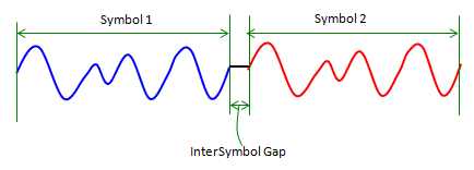
Figure: Inter-Symbol Gap in OFDM
There is a big benefit in using large symbols as shown in the above figure. It is now possible to leave a relatively large gap between successive symbols without losing too much link capacity. As long as this gap is larger than the path length (in time) of longest multipath signal, the OFDM system will be immune to Inter Symbol Interference. The inter-symbol gap is not left empty, but instead the last portion of the next symbol (equal to the length of the gap) is inserted there, and this technique is known as the Cyclic Prefix Extension.
Consider the following example: If we were to transmit a million symbols per second using single carrier QAM modulation, then the duration of each symbol would be one microsecond or less. If the same million symbols per second are spread among one thousand OFDM sub-carriers, then the duration of each symbol will be longer by a factor of a thousand (i.e., one millisecond) with approximately the same total bandwidth used. Assume that an inter-symbol gap or guard interval of 1/8 of the symbol length is inserted between each symbol. Inter Symbol Interference can be avoided if the multipath time-spreading (the time between the reception of the first and the last echo) is shorter than the guard interval (i.e., 125 microseconds). This corresponds to a maximum difference of 37.5 kilometers between the length of the main signal and its largest multipath component.
4G LTE uses a symbol time of 66.7 us and a Guard Interval of 4.69 us, which allows the system to accommodate path variation of up to 1.4 km, which is good enough for densely deployed LTE cells.
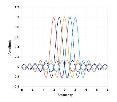
Figure: OFDM Sub-Carriers
Note that it is no longer necessary to shape the transmit pulses into the shape of a sinc in order to avoid Inter Symbol Interference (since interference is avoided by using the Guard Interval), hence the transmit signal can be a square pulse for each sub-carrier. As a result, the shape of the per carrier frequency response is in the form of a sinc function. This is illustrated in the above figure which shows the spectrum for a full OFDM symbol, consisting of multiple subcarriers. Each of the subcarriers assumes a sinc shaped spectrum as shown, and since they are spaced apart from each other by a multiple of a frequency, it results in the shape shown. Note that unlike in regular single carrier based Frequency Division Multiplexing, it is not necessary to leave a guard band between sub-carriers, since they don’t interfere with another due to the orthogonality property.
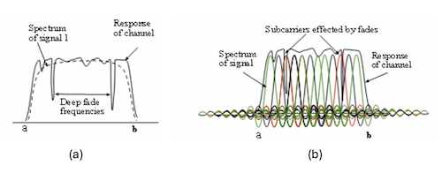
Figure: Frequency Selective Fading in an OFDM System
Part (a) of the above figure shows the frequency response of a channel undergoing frequency selective fading (the solid line). If we use Single Carrier Modulation QAM in such a channel, then its frequency spectrum spans the entire channel bandwidth, and as a result, the frequency selective fading can cause a whole symbol to be lost. On the other hand, as Part (b) of the figure shows, with an OFDM system, the portions of the spectrum that are affected by the frequency selective fades, are localized to only a few of the subcarriers in the OFDM signal, which makes the transmission much more robust compared to single carrier systems. Since we are allowed to use different modulation schemes on different sub-carriers, the part of the spectrum which is subject to fading can adaptively change its modulation to a something more robust such as QPSK, or even refrain from using the affected sub-carriers.
In some sense OFDM is a logical inverse of single carrier based modulation, since
- Single carrier modulation QAM leads to a sequence of tiny pulses in time, that are tightly stacked next to each other and kept orthogonal by using the sinc function AND these pulses have a wide spectral band in the frequency domain. Furthermore neighboring spectral bands are kept orthogonal by leaving a gap in-between them.
- OFDM modulation leads to a sequence of tiny sub-carriers in frequency, that are tightly stacked next to each other and kept orthogonal by using the sinc function AND these sub-carriers have a wide pulse in the time domain. Furthermore neighboring time pulses are kept orthogonal by leaving a gap in-between them.
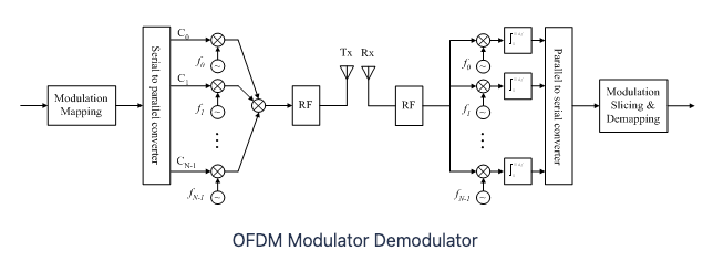
Figure: The OFDM Transmitter and Receiver
The above figure shows an OFDM transmitter and receiver. On the transmit side it shows the serial bit stream getting mapped to N single carrier QAM symbols. Note that we can use a different modulation for each sub-carrier, so far example if sub-carrier 1 is using 256-QAM then 8 bits get mapped to each of its symbols, while if sub-carrier 2 is using QPSK (since it is in a more challenging part of the channel spectrum) , then 2 bits get mapped to its symbol. The individual single carrier symbols QAM are then added together to generate the OFDM symbol that then gets transmitted over the channel (after shifting the subcarriers to a higher part of the spectrum in the RF block). On the receive side the signal is first decomposed into its individual components by multiplication with the N subcarriers in parallel. This is followed by a parallel to serial converter and the detection block in which the transmitted bits are recovered.
OFDM Implementation Using the Discrete Fourier Transform
The OFDM Transmitter and Receiver systems that were shown at the end of the last section have a very big problem: They are basically un-implementable! The reason for this is that they require as many oscillators as there are sub-carriers in the system, and given that a realistic OFDM system can have hundreds if not thousand of sub-carriers, implementation can get very expensive.
So what is the way out? Well, once again the Fourier Transform comes to the rescue, this time in the form of the Discrete Fourier Transform or DFT. As we show next, DFT allows us to replace the operation of multiplying with a sine or cosine signal, with that of computing the DFT or the inverse-DFT, which is much easier to do. This critical idea was first fully developed by Weinstein and Ebert at Bell Labs in 1971, five years after the original OFDM paper by Robert Chang. Bell Labs however did not show much interest in this technology, and the first commercial implementation had to wait to 1993, with the start-up Amati Networks who applied OFDM to ADSL transmissions, which take place over Twisted Pair copper wiring.
In order to see how DFT can be applied to OFDM, lets start with the OFDM Transmitter that was shown in the previous section. The following equation captures the generation of the baseband signal:
\[x(t) = \sum_{n=1}^{N} A_n\ e^{j2\pi nt\over T}, \ \ \ 0\le t\le T\]Note that the sequence $A_n, n=1,…,N$ is the set of complex numbers that captures the type of QAM modulation being used. These then get multiplied by the set of N discrete carriers at frequencies ${n\over T}, n= 1,…,N$ and added together to generate the OFDM baseband pulse.
We are now going to sample the baseband pulse $x(t)$ N times, at time instants $t = {T\over N}, {2T\over N},…,{(N-1)T\over N}, T$, thus generating N samples $x_k, 1\le K\le N$. Substituting these in the equation for $x(t)$, it follows that the samples satisfy the following equation:
\[x_k = \sum_{n=1}^{N} A_n\ e^{j2\pi nk\over N},\ \ \ 1\le k\le N\]This is where magic happens! If you go back to the section on the Discrete Fourier Transform, you will notice that these equations are exactly the same as for the Inverse DFT for a signal whose frequency samples are given by $A_n, 1\le n\le N$. Hence we have avoided the use of all the oscillators in the generation of an OFDM pulse, simply by discretizing the signal and using the inverse DFT to generate its samples. This observation provides a straightforward way in which the numbers $A_n$ can be recovered at the Receiver, simply carry out the inverse operation (which is just the regular DFT), and these numbers re-appear!
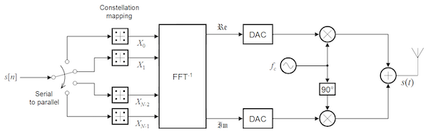
Figure: OFDM Transmitter Implementation using an Inverse Discrete Fourier Transformation
But before we can do that, we have to transmit the signal over the analog channel, and in order to do this we will have to transform the samples $x_k, 1\le k\le N$ into an analog pulse. This is done using a Digital to Analog Converter (DAC) as shown in the above figure, and is done separately for the Real and Imaginary components. The resulting two analog signals are then multiplied by the carrier wave at frequency $f_c$ to generate the passband signal $s(t)$ that is transmitted over the channel.
\[s(t) = \Re[{e^{2\pi f_c t} x(t)}], \ \ \ 0\le t\le T\]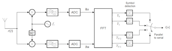
Figure: OFDM Receiver Implementation using a Discrete Fourier Transform (DFT)
The received passband pulse $r(t)$ is given by
\[r(t) = s(t) + n(t),\ \ \ 0\le t\le T\]where $n(t)$ is the channel noise. The received signal can be shifted to the baseband as follows
\[y(t) = r(t) e^{2\pi f_c t},\ \ \ 0\le t\le T\]Note that the signal $y(t)$ has a real and imaginary part, and each of these sent through a Analog to Digital Converter, to generate a complex valued discrete sequence $y_k, 1\le k\le N$. Subsequently DFT is used to recover the complex valued QAM symbols $A_n, 1\le n\le N$, given by
\[A_n = {1\over N}\sum_{k=1}^{N} y_k\ e^{-j2\pi nk\over T},\ \ \ 1\le n\le N\]These QAM symbols are then sent to a Symbol Detector to regenerate the bit sequence corresponding to each symbol.