Latent Spaces: Capturing Structure in Complex Systems
Introduction
A few years ago, the late physicist Freeman Dyson wrote an essay titled “Why is Maxwell’s theory so difficult to understand?”, in which he made the interesting observation that Electromagnetic theory presents a picture of the world with two layers. The first layer, which consists of the Electric and Magnetic fields that make up the theory, is entirely described using mathematical equations that govern these fields, how they interact with each other and how they evolve over time. The quantities in this layer, namely the aforementioned fields, are abstract in nature and not accessible to our senses. The second layer on the other hand, consists of quantities such as charges, current, energy and forces that we can directly measure, and are a part of our world. This two-layer structure is useful since it turns out that a mathematical description of the second layer in itself is intractable, but the second layer quantities can be computed from the abstract first layer quantities. Furthermore, the first layer lends itself to a mathematical description (the Maxwell’s Equations of Electromagnetism), which though complex, is still tractable. Dyson further observed that Quantum Mechanics, whose equations were discovered about 60 years after Maxwell’s Equations, also shares this two-layer structure. In this case the first layer consists of quantities such as the Schrodinger Wave Function or Quantum Fields that are once again inaccessible to our senses and measuring instruments, but nevertheless lend themselves to a mathematical description. The second layer consists of predictions about the structure of atoms, molecules and atomic processes which can be computed from the first layer quantities by using the equations of Quantum Mechanics and verified using experiments. Once again, a direct mathematical description at the atomic level of the second layer using quantities that we can measure, such as position and momentum, is intractable.
For both Electromagnetism and Quantum Mechanics, the fundamental physical processes happen in their respective first layers and are hidden from us. Scientists have tried to create a understandable model of the first layer in terms of processes and objects that are familiar to us. For example, Electromagnetic Fields were initially modeled using a mechanical system consisting of springs while attempts have been made to model Quantum Mechanics using familiar objects such as particles and waves. However, in both cases the attempts have been unsuccessful. Dyson makes the point that the first layer is an entirely mathematical construction, and it doesn’t make sense to try to reduce it to descriptions that make sense in the macro world that we live in since our language was not designed to describe the layer one processes. The main utility of the first layer is to provide a mathematically tractable model from which predictions about events in the real world can be made with a high degree of accuracy. The process by which the real world in the second layer manifests itself from the processes happening in the first layer remains largely mysterious, and in the context of Quantum Mechanics goes by names such as Quantum Wave Collapse or Quantum Decoherence.
My objective in this essay to explore the existence of this two-layer structure as a common organizing principle that is used to structure other complex systems, in particular we will look at two broad domains, namely Biology and Deep Learning systems. In Biology, an organism’s DNA can be considered to be the first layer structure, which by itself is fairly simple to describe, but when expressed in the language of proteins and cells by using the Genetic Code, it results in the complex second layer structure and multiplicity of living things that we find around us. The cellular ‘decoder’ used to translate the layer one structures in the DNA into layer 2 structures of animals and plants is beginning to be understood thanks to the progress in Biology over the last seventy years. This decoder is itself subject to change over time, using the Law of Natural Selection as first discovered by Charles Darwin, resulting in new species of plants and animals. These laws are reasonably simple, hence are comprehensible to us, and yet they result in complex Biological structures whose origin was completely mysterious before Darwin came along.
In this essay I will show that modern Deep Learning systems also obey the two-layer design principle for complex systems. In this case the first layer typically goes by the name of Latent Variables. Once again, these live in multi-dimensional spaces called Latent Spaces that consist of hundreds of dimensions and are not comprehensible to our senses, but they capture the structure present in objects in the real world, which form the second layer of the structure. The Artificial Neural Network serves as a system to translate the abstract first layer latent variables into concrete objects such as images and language that we can comprehend. These Artificial Neural Networks, that go by names such as Convolutional Neural Networks and Transformers, were originally inspired by models of how the human brain operates, even though the underlying mechanisms are very different in the two cases. By playing around with the Latent Variables we are able to carry out complex manipulations of images and text that was not possible before. Moreover, we can solve the difficult problem of translating between dissimilar datasets by establishing a correspondence between their Latent Spaces, an example of which is generating an image by describing it in words.
This also raises the interesting question of whether the brain itself is organized according to the two-layer design principle. It could be that information is organized in the brain in multi-dimensional layer one structures, which are then converted into the three dimensional space and time that we perceive and words that we understand, using the brain’s Neural Network.
Latent Vectors and Latent Spaces in Machine Learning
A Latent Vector is a point in n-dimensional space which is obtained as a result of mapping a real world (or layer 2) object, such as images or text, using an Artificial Neural Network (ANN). Hence this can be written as:
\[f_{ANN}(image) = (x_1,x_2,...,x_N)\]or
\[f_{ANN}(text) = (x_1,x_2,...,x_N)\]where the function $f_{ANN}$ represents the Artificial Neural Network or ANN (see Fig. 1 below). The Latent Vector by itself is not that interesting, the magic happens when it is used to carry out useful operations, such as classification or prediction. Indeed, Latent Vectors in combination with their ANNs can be used to generate novel layer 2 objects, an area which is referred to as Generative AI. We will see later in this essay that Latent Vectors can also be used for control or optimization of the real world objects that they represent. We will see that Latent Vectors can be considered to be a layer 1 abstract representation in the sense that Dyson talks about, with the images or text serving the layer 2 objects that exist in the real world.
Given a dataset consisting of images (or text), the set of all such points of Latent Vectors forms something called a manifold, which is a complex geometric structure in N-dimensional space, and is referred to as Latent Space. The power of the Latent Space concept lies in the fact that it is able to capture structure that’s present in the layer 2 datasets. This structure was hidden from our comprehension before the advent of ANNs, whether in images or in language, but becomes apparent when the data is translated into Latent Vectors. It is often tied to the semantic content in the datasets and is too complex to capture with the usual tools of mathematical analysis.
One of the early observations in Deep Learning was that images that are similar to each other or text that has similar meaning result in Latent Vectors that lie close to each other in Latent Space, which makes is easier to do classification. The use of Latent Vectors for control also relies on the property that input states with similar control signals cluster together. Moreover, by establishing a correspondence between Latent Spaces from dissimilar datasets, such as images and text, it is possible to translate from one dataset to another. This property drives models such as Open AI’s DALLE 2, that generate images from text descriptions.
The most fascinating aspect of Latent Spaces is that Latent Spaces for images and text are the same at a very fundamental level. In other words, one can start from a Latent Vector and use it to generate either an image or piece of text (using different ANNs), and both of these will be semantically equivalent. This magic is done by taking the two Latent Spaces and establishing a correspondence between a few of their Latent Vectors, with the hope that the remaining Latent Vectors will also match. This would not possible unless the image and text Latent Spaces are topologically similar (or isomorphic).
The ANNs that encodes the layer 2 dataset in some sense extract the deep structure present in the data, which enables them to compress it down to its essentials, and this representation is the Latent Space. Until now datasets were represented by statistics like the average or standard deviation, or if more ambitious its higher moments. But clearly we now have a better way of representing datasets. Once we have a Latent Space representation, we can do things that were impossible to do before, including generating new samples similar to the ones in the original dataset (which goes back to Feynman’s quote “I truly don’t understand something unless I am able to make it myself”). Such a representation was not possible before, and its implications are still percolating through Science, Engineering and even the Humanities. In addition to text and images, there are other complex systems over whom we have limited control since our understanding of their deep structure is limited, such as the Economy, Financial markets etc. If we can represent them as Latent Variables, it gives us a handle that can be used to better understand and control them.
Latent Space for Images
As a result of advances in Deep Learning in the last decade, we now have the technology to be able to conjure up images by simply describing them in words, or manipulate an image by using simple mathematical operations. But how did we get to this point? Not too long ago, the only way to manipulate images was by modifying the hundreds of thousands of color pixels that make up an image, which is a complex undertaking. Clearly images have a lot of underlying structure, which should help in manipulating them, but we had no way to access this structure. Examples of such structures could be: A car image is made up of a chassis, which is turn has components such as doors, windows, seats etc. or a human image is made up limbs, head, face, etc. and the face in turn has eyes, lips, nose etc. while limbs have joints, toes and fingers. Thus what was missing was a semantic level understanding of images, which could allow us to discover similar images or manipulate it.
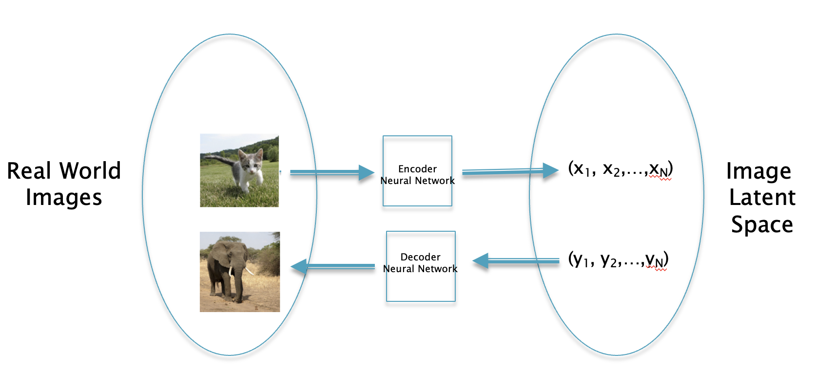
Figure 1: Mapping between images and their Latent Vectors
Fig. 1 shows a mapping between images and their Latent Vector representations. The image itself is described by three 2D planes of red, green and blue pixels, and each pixel is represented by a number between 0 and 255. The Latent Vector representation on the other is just a N dimensional vector. The magic lies in the ANN that converts the image to its corresponding Latent Vector, and is also able to convert a Latent Vector back into an image. The Latent Vector is the hidden layer 1 representation of the image and it can be used to carry out image manipulation tasks that were impossible to accomplish before the advent of Deep Learning.
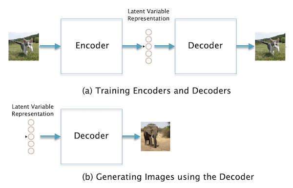
Figure 2: Generating Latent Vectors for images
Part (a) of Fig. 2 shows a block diagram of how an ANN is trained to generate Latent Vectors. In general there are two Neural Networks involved, the Encoder network takes an image and converts it into a vector, while the Decoder network does the reverse operation in a such a way such that the original image is recovered. Once the Encoder and Decoder have been fully trained (using a training dataset with millions of images), the Decoder by itself can be used to generate new images, as shown in Part (b) of the figure. From this description it is clear that fundamental to the operation of this system is the idea of compression, since the Encoder takes an image consisting of hundreds of thousands of pixels and converts it into a vector with a few hundred numbers. In order to do so the Encoder has to capture the essence of the image, both the semantics (the shapes of the objects in the image and their relationships) and the texture (colors etc.), and do it in such a way that all extraneous information is filtered out.
Over the course of the last decade, the Encoder and Decoder ANNs have become more sophisticated resulting in better quality of the generated images. Initially they were simple Dense Feed Forward Networks, and later the discovery of Convolutional Networks (CNNs) led to big jump in performance. The latest ANNs employ a technique called Diffusion Models in the Decoder which has led to the creation of State of the Art systems like DALLE 2.
What is the theoretical basis for believing that an invertible Latent Vector representation for images is even possible? At a fundamental level, the ANN is able to capture the probability distribution of the pixels in the images. This is an unimaginably complex function, which we were unable to access before the advent of ANNs. It has millions of parameters that are stored as weights of the ANN, which means that the network itself is the representation for the probability distribution function. Hence we no longer have a simple mathematically tractable representation for the probability distribution function, but it is nevertheless accessible through the ANN. The Decoder inverts this distribution function in order to sample from it, which results in the generation of new images. As Neural Networks have improved and become more sophisticated, they have been able to capture more complex functions and as a result the quality of images that they are able to generate has become better.
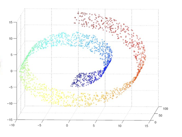
Figure 3: Visualization of a Latent Space manifold
The set of Latent Vectors for an image dataset lie on a structure in N dimensional space called a manifold. A manifold is defined as a surface in N dimensional space that can be locally approximated by Euclidean space. Moreover, given two Latent Vectors on a manifold, the points on the linear segment connecting them also lie on the manifold. The manifold doesn’t lend itself to easy visualization given that it lies in N dimensions, however for the case N = 3 the the manifold can be visualized, and one such object is shown in Fig. 3. Latent Vectors for a particular class of images get mapped close to each other in the Latent Space, and are shown with their coloration.
There is a technique that sometimes helps in visualizing Latent Space manifolds in higher dimensions, and this is discussed next.
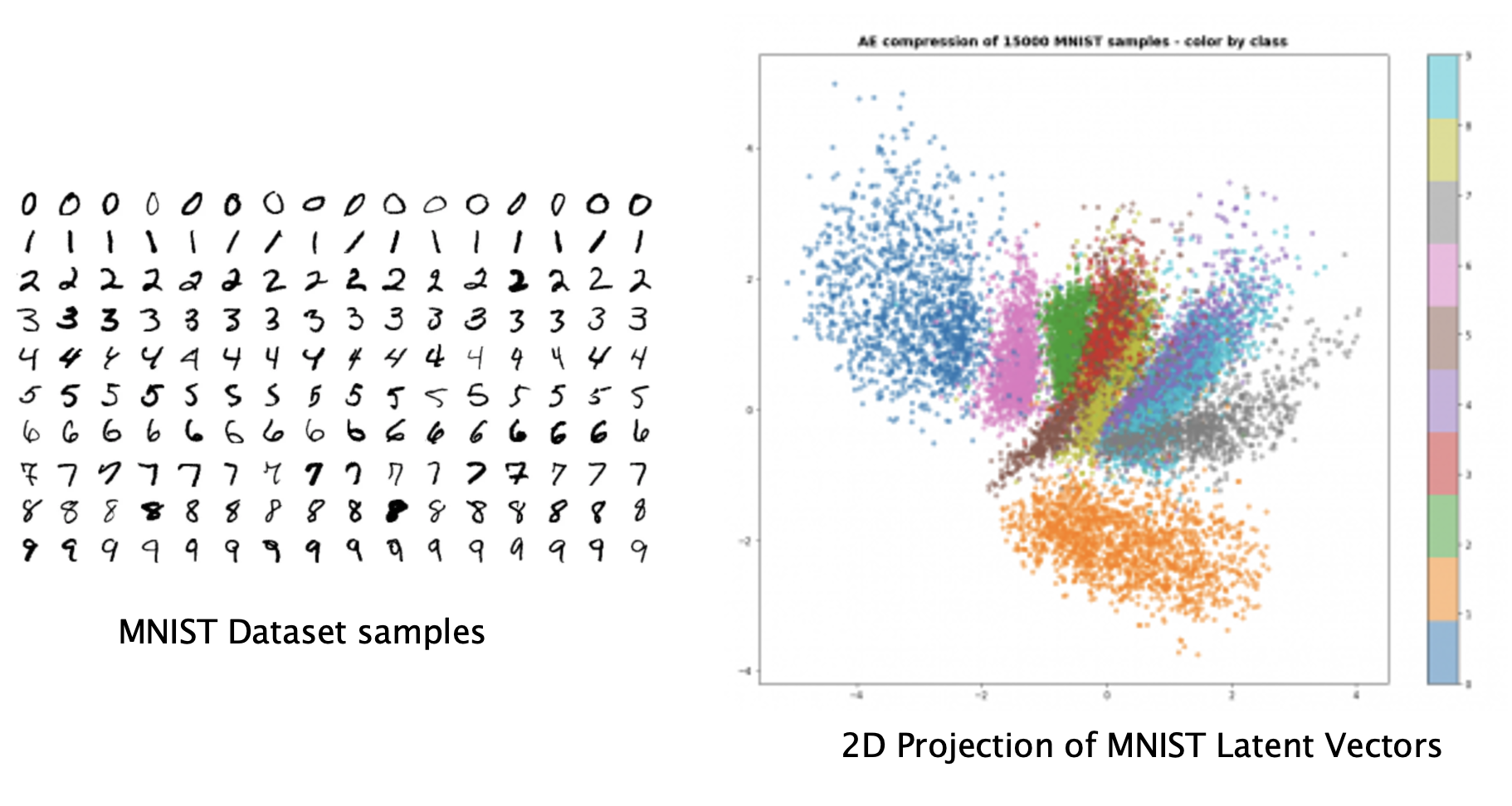
Figure 4: Projection of the MNIST Latent Space manifold on to 2D space
The MNIST image dataset consists of handwritten digits from 0 to 9 and has been extensively used from the earliest days of Deep Learning. Some samples from this dataset are shown in the LHS of Fig. 4. Latent Variables for this dataset were obtained using a type of ANN called Variational Auto Encoders, and then these were projected onto 2 dimensions using a technique called T-SNE (see RHS of figure). The 2D projection makes the structure of the MNIST Latent Space much more comprehensible to us. The Latent Vectors for each of the 10 digits form distinct clusters (shown in different colors) which shows that the ANN has managed to figure out that there are ten semantically distinct types of objects in the dataset. We can also see why this representation makes it much easier to classify digits which we can do by simply by finding the cluster within which its Latent Variable is located.
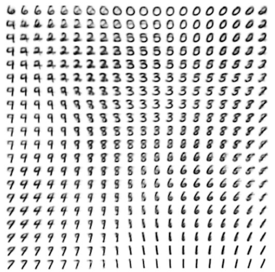
Figure 5: Interpolation between images
Now that we have a Latent Variable representation for an image, there are several interesting things that can be done with it. Fig. 5 shows how we can interpolate between images, once again using the MNIST dataset as an example. The numbers 6, 2, 7 and 1 form the four corners of the grid, and if these are converted into their Latent Variables, we can interpolate between images by interpolating between their Latent Variable representations, and then converting the interpolated vector back into an image.
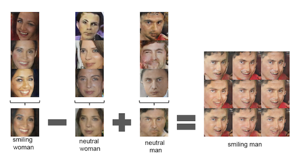
Figure 6: Manipulation of images by doing vector arithmetic in Latent Space (from Radford et.al)
Another interesting way of manipulating images is shown in the Fig. 6: If the Latent Vector for an image of a smiling woman is subtracted from the Latent Vector of an image for a neutral woman, and the result is added to the Latent Vector for an image of a neutral man, then the resulting Latent Vector can be decoded into an image of a smiling man (to be more precise, the Latent Vectors on the LHS were created by averaging the Latent Vectors of several similar images). This shows that encoded within their array of numbers, Latent Vectors carry semantic information about images, .
Latent Space for Text
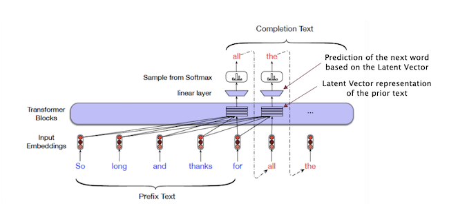
Figure 7: Text generation using a Language Model (from Jurafsky and Martin)
Latent Vectors for text are computed using Language Models such as GPT. The generation of new text is done on a word by word basis with word $n$ and prior words being used to predict the following word $n+1$ (the analogous procedure for images would have generated them on a pixel by pixel basis, which is indeed possible, but time consuming). Fig. 7 shows a trained Transformer model which is tasked with completing the phrase “So long and thanks for”. This phrase is fed into the model, which then starts to generate the following words to complete the phrase, one at a time. In order to do so, the model computes a Latent Vector representation for all of the prior text, which is then decoded by a Logit Layer to predict the next word.
What is the nature of the information captured in this Latent Vector which enables it to do such a good job of next word prediction? The information encoded in the Latent Vector for languages is quite complex, and the answer to this question is still being researched. Li et.al. investigated this question for the simpler case of the board game of Othello, in which they replaced words by the game moves and fed them into a Transformer model on a sequential basis. They probed the Latent Vector that is used to predict the next move, and showed that the state of the Othello board could be recovered from it. This implies that the Latent Vector encodes the current state of the game, even though this information was not fed into it explicitly. It is thought that Language Models such as GPT, which are fed enormous quantities of text data during their training, perhaps incorporate a model of the real world in their Latent Vectors. This could be a byproduct of the process of encoding all of the training data, in the most efficient way possible.
Translation between Datasets using Latent Variables
One of the most fascinating discoveries of the Deep Learning era is the realization that we can map between very dissimilar datasets by connecting their Latent Spaces together. Indeed one can consider that the datasets share a common Latent Space, i.e., it is possible to start with a Latent Vector and generate a sample from either Dataset 1 or Dataset 2, depending upon the ANN deployed as the decoder. In language translation applications a sample from Dataset 1 is converted into its Latent Vector representation, which is then directly used to generate a sample from Dataset 2.
The power of the Latent Space formulation is most evident when we try to solve the problem of translating between datasets that are very different from each other at the layer 2 level. However it turns out that if they share a similar structure at the deeper Latent Space or layer 1 level, then it is possible to ‘translate’ an object in dataset 1 to a corresponding object in dataset 2 in a way that makes sense to us. The most common example of this is translating a piece of text to an image that is described by the text. Other examples include:
- Translating from image to text, also known as captioning
- Translating text from Language 1 to Language 2
- Translating from Image Class 1 to Image Class 2: For example converting satellite photos into road maps
- Converting a piece of text to its summary
- Answering a question (which is the same as translating from a question to its answer)
The class of such problems, which also go under the name of Generative AI, had been very difficult to solve using pre-ANN methods.
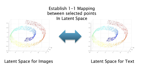
Figure 8: Establishing a 1-1 mapping between two Latent Spaces
Fig. 8 summarizes the main idea behind inter-dataset translations, as applied to text and image datasets: Each of these datasets has its own Latent Space and during the training process, we establish a correspondence or mapping between points in the two spaces. This is done explicitly using algorithms such as CLIP, or implicitly as part of the training process that is used to convert from text to images. Once the Latent Vectors in the Training Datasets get mapped, the rest of the vectors in the two Latent Spaces are also get mapped by the process of interpolation (assuming that the Latent Spaces share a common structure).
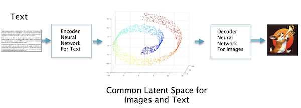
Figure 9: Converting a piece of text to an image
Once the mapping is established, translating a piece of text to an image can be done by generating Latent Vector 1 for the text sample, and then using this to generate the corresponding Latent Vector 2 for an image that is closest to it (in practice this is done automatically by the generating Neural Network). Latent Vector 2 is then used to generate the image we are looking for.
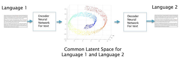
Figure 10: Translating between languages
If the two Datasets have the same modality (for example image to image or text to text), then this procedure establishes a correspondence between two versions of the same Latent Space as shown in the Fig. 10.
Before the advent of modern Neural Networks, it was not thought possible to translate from a Latent Vector representation to full fledged image or a piece of text that is semantically coherent due to the complexity of the mathematical transformation required. Deep Learning has shown us a way of learning these fantastically complex functions, and as result we are able to generate samples from datasets which were previously the domain of human level intelligence. The Latent Spaces themselves have some complex topological structure about which we know very little, but the fact that image and text Latent Spaces can be put into one-to-one correspondence seems to imply that at the very deep level they are identical. This is plausible when two Latent Spaces are from different languages, and this fact is used to do language translation. However the fact that images and text are also deeply connected at the Latent Space level is, in my opinion, one of the important discoveries that has been made thanks to Deep Learning, and it has implications in the study of how information is stored in the brain.
The technique of establishing congruences between dissimilar datasets at the Latent Space level, and using this property to translate between them, is in its early stages and can be extended in a number of different directions. One possible extension is translating between digital datasets and objects in the real world. In a later section I will argue that living things are an example of such a translation, between the Latent Space of DNA and our bodies and organs.
Control in Latent Space
In the previous section we showed how the difficult problem of translating between dissimilar datasets is solved by establishing a correspondence between their Latent Spaces. There are other intractable problems whose solution is simplified by operating in their Latent Spaces, and in this section we consider the problem of Control.
One way of formulating the problem of Optimal Control is as a multistep problem, where an Agent tries to maximize an objective, usually called a Reward. At each step the Agent has access to the state S of the world in which it operates, and has to decide to take one of several actions A that are available to it. Furthermore the Agent’s action causes the state S of the world to change in an unpredictable way. The Agent’s action A can be formulated as a function f of its current state S, so that $A = f(S)$, for a class of control problems called Markov Decision Processes.
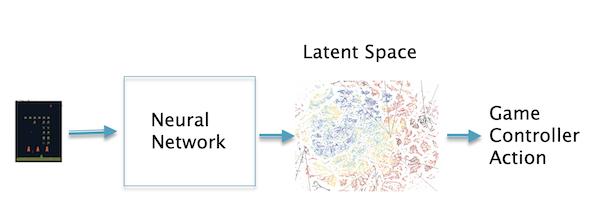
Figure 11: Using Latent Variables for Control
For the case when the control actions are based on visual information from the real world, the state S can be simply considered to be the images being fed to the agent from a camera, such a setup is appropriate for the problem robotic control for example. Before the advent of Deep Learning it was not possible to feed such a complex state to the agent, usually the information in the image was condensed into a few numbers that the agent could handle. Deep Learning systems on the other hand are able to process the hundreds of thousands of pixels in images, and derive control information from them. This is shown in the Fig. 11 for the case of Video Game control in which the agent generates game controller actions from the state information in the game screen. Once again the Latent Space plays a critical role by serving as the condensed representation of the structure present in the images, as specialized to the task of control. The control actions can be directly mapped to the Latent Space, such that images that have the same control action are clustered together. The feasibility of this system was first demonstrated by DeepMind in 2012, using an algorithm that they called DeepQ.
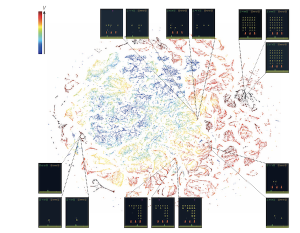
Figure 12: The Latent Space for Screens Shots for the Atari game of Space Invaders (from Mnih et.al.)
An example of this Latent Space for the Atari game of Space Invaders in shown in Fig. 12 (after being mapped into 2D space using the T-SNE method). Each point in the graph corresponds to a Latent Variable representation of one of the Game Screens, while its color corresponds to something called a Value Function, which is the system’s estimate of the Reward that it may get during the game. This graph clearly shows that the ANN has been able to find a structure in the game screens as a function of the ‘Reward that the screen generates’. This enables it to classify the game screens such that screens that have similar Rewards cluster together in the Latent Space.
Optimization in Latent Space
In this section I am going to summarize some interesting research that was recently published by Qi et.al., where they utilized ANNs to find the crystal structure for a chemical formula that has minimum formation energy, and thus corresponds to a stable material. This is an important problem with applications to problems such as drug or protein design and also serves as an example of an optimization problem that becomes simpler to solve in Latent Space.
In this application, the input into the model consists of the chemical formula for the compound and the output is a three dimensional crystal structure for that compound that has the minimum formation energy. Finding the optimum crystal structure is a difficult problem in the 3D space of full molecular structure, but becomes simpler when carried out in Latent Space. This is also an example of using the concept of Latent Space in fields other than text or images.
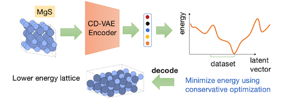
Figure 13: Optimization in Latent Space (from Qi et.al.)
The most straightforward way of approaching this problem is by computing a formula for the formation energy based on candidate crystal structures for the compound and then choose the structure with the lowest energy. However this procedure requires optimizing over complex sets and non-Eucledian manifolds so that naively applying gradient based methods to do optimization does not usually result in improvements. Qi et.al. proposed an alternative optimization approach which overcomes these challenges. As shown in the Fig. 13, their idea is to do optimization in the Latent Space of crystal structures, as opposed to the structures themselves. The crystal structures are converted into Latent Vectors using a Crystal Diffusion Variational Autoencoder (CD-VAE), which are then optimized using a simple. gradient based algorithm. The ANN that they used was borrowed from those used to encode and decode images, such as Convolutional Neural Networks. Once the Latent Vector with the lowest formation energy is identified, it is converted back into the 3D crystal structure using a Diffusion Model (similar to those for used DALLE 2 or Stable Diffusion for image generation).
DNA: Latent Variable for Living Things?
In this section we step away from the field of Machine Learning and look for evidence of Latent Vector like structures in other fields, starting with living things. It was not that long ago that scientists discovered that the incredible variety of plants and animals on earth all shared a common molecular structure in the nucleus of each of their cells which they called DNA. Since then a lot has been discovered about how DNA helps our cells function so that we stay alive, and also how it helps build our bodies. It is the latter function that we will focus on in this section. We will argue that the process of building an animal body using DNA can be likened to the way in which the decoder in a Machine Learning system converts a Latent Vector into text or an image.
We now know the following about how DNA works:
- DNA is a linear code made up of an alphabet consisting of 4 chemical bases, referred to in short as A, G, C and T. Each DNA strand consists of a linear sequence of millions of these four bases.
- There are discrete portions of the DNA called genes, and living organisms typically have tens of thousands of genes in their DNA. The coded sequence in a gene gets translated into a protein, using the Genetic Code, which is a mapping of four consecutive bases in the gene to one of twenty Amino Acids. This process is accomplished by means of translation (also called transcription) of the information in a gene to Messenger RNAs, which are turn is processed by Ribosomes in the cell to make proteins. Proteins are the fundamental building blocks of life and driver of all chemical processes that build the animals body and also keep it alive.
Since the 1980s we have learnt a lot about how genes control the development of our bodies from the time we are embryos, and this is the part that is of interest to us in this section. Most of the content described on this topic is from the excellent book “Endless Forms Most Beautiful: The New Science of Evo Devo” by Sean B. Carroll and is summarized next.
Even before the 1980s it was clear that genes somehow were responsible for influencing the shape and structure of our bodies, but it was a mystery how they went about the job. It was known that humans and chimpanzees share 98% of their genes, even humans and rats share around 80%. Hence it was perhaps not the genes themselves but some other unknown factor that took a similar set of genes and fashioned them into different species of animals.
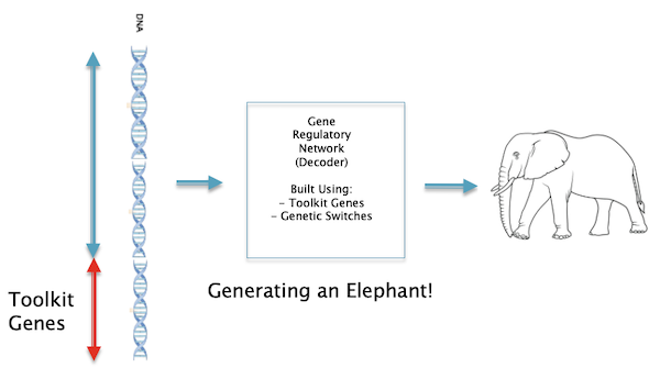
Figure 14: Building an elephant using the Gene Regulatory Network
The missing factor was discovered thanks to experiments carried out on the fruit fly Drosophila, and is referred to as the Gene Regulatory Network (GRN). A high level view of how this network functions is shown in the Fig. 14. Just like the Decoder in Machine Learning systems, the GRN also functions as a Decoder network which takes the information coded in the genes and generates an animal from it. The structure of the GRN is coded in the DNA itself and is built using two main ingredients:
- There is a set of genes in the DNA which are called Toolkit Genes. The main function of these genes is to switch other genes On and Off, and the toolkit genes themselves can be switched On and Off (by other toolkit genes). Amazingly enough these genes are common across animals as diverse as fruit fly’s and humans separated by hundreds of millions of years of evolution. There are a few hundred of these genes out of the approximately 13,000 in the fruitfly.
- Every gene in the DNA has associated stretches of DNA which have the capability to turn the gene On or Off, these are known as Genetic Switches. In general there are multiple Genetic Switches controlling each gene.
The combination of the Toolkit Genes and Genetic Switches are responsible for building the animal’s Gene Regulatory Network. This system of Toolkit Genes and Genetic Switches was put in place in the early pre-history of animals more than 600 million years ago, in a period known as the Pre-Cambrian, and has functioned with only a few changes since then. New species of animals are generated by making changes in the Gene Regulatory Network and these are governed using the Laws of Natural Selection. These changes happen more commonly in the Genetic Switches as opposed to the Toolkit Genes.
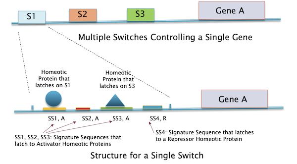
Figure 15: How Gene Transcription is Controlled using Gene Switches
Fig. 15 shows in more detail how genes can be turned on or off by means of a Gene Switch which is a stretch of DNA in front of a gene. There can be multiple switches controlling a single gene, one of which is expanded in the lower part of the figure. Each switch in turn contains a number of gene sequences called Signature Sequences, and these act as attractors for the proteins produced by the Toolkit Genes (called Transcription Factors). These proteins latch on to the Signature Sequence of the switch and this can result in either turning on the expression of that gene or turning it off. In general there can be multiple Signature Sequences in each switch, each associated with a different Transcription Factor.
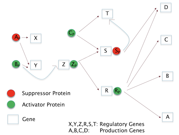
Figure 16: A Gene Regulation Network
These Transcription Factor proteins in turn can be controlled by other Transcription Factor proteins, and this enables this system of proteins and switches to form a sophisticated logic network that can be used to control the operation of genes very precisely, as a function of time and space and this forms the GRN. An example of such a network is shown in the Fig. 16. Carroll estimates that about 100 pages are probably sufficient to write down the GRN for the fruitfly, while for a human it would be closer to 10,000 pages.
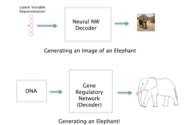
Figure 17: Generating an image of an Elephant vs Generating an actual Elephant!
To summarize: There is a direct analogy between Neural Network Decoders and the GRN, as well as between a Latent Variable representation and the DNA. The space of DNA sequences for a particular species, for example humans, forms a Latent Space, and one can consider all possible humans who have ever lived, as well as those that might live in the future, to be samples from this Latent Space.
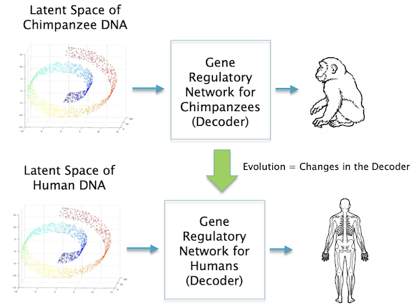
Figure 18: Difference between species are mostly due to differences in the Gene Regulatory Network
There is an interesting difference between the Decoders for two cases: ANN decoders are designed by us, and have gradually become more sophisticated over time as we have become better at designing Neural Networks. Biological Decoders on the other hand are made by the same basic substrate, i.e. the animal’s DNA, and also changes over time leading to new animal species. But now there is no designer other than the laws of Natural Selection as shown in the Fig. 18.
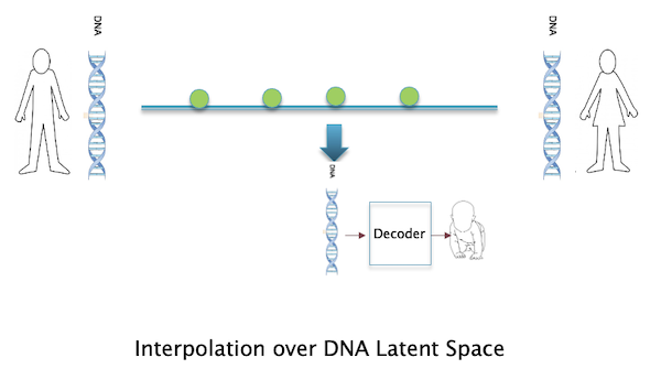
Figure 19: Interpolation between Latent Variables in DNA Space
Just as we can interpolate between Latent Variables in Machine Learning to produce images that are intermediate between the two end points, one can consider the process of animal sexual reproduction to be a type of interpolation in the DNA space (see Fig. 19)!
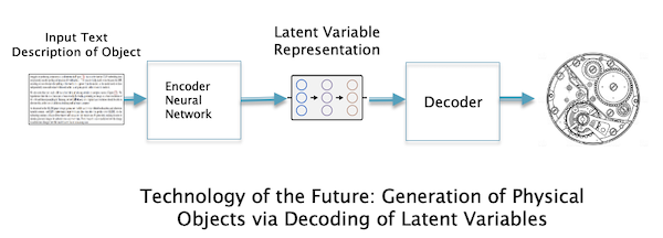
Figure 20: Technology of the Future: Generation of Physical Objects from Latent Variables
If we consider the Gene Regulatory Network in animals to be a type of very advanced technology (invented 600 million years ago!), then there are lessons that we can draw to apply to our current generation of Neural Networks. Here are some ideas:
- Invention of Decoders that can generate not just text or images, but also physical objects (see figure). Perhaps very intricate machinery or micro-machinery in the future can be manufactured using such a technique.
- Use Latent Variables to generate the Decoder itself. The Latent Space of Decoders can be explored separately from that of text or images, and some kind of optimization procedure, analogous to Natural Selection, can be used in this space to generate better Decoders.
There is also an interesting analogy between how animal bodies develop and how images are gradually produced from noise in a decoder based on Diffusion Models:
- The development of an embryo follows a process whereby the animal’s body plan is first mapped out using Toolkit Genes, such that the cells in every part of the growing body know exactly their location with respect to the overall plan. Once this is done then the cells in the various locations differentiate themselves based on their location, and result in the development of body parts or organs that are specific to that Location.
- The development of an image using Diffusion Models also follows a two-stage process where the overall semantic content of the image is first laid out, this includes the shapes of the objects in the image and their relative locations. This is followed by the filling in of details in the image, such as colors and textures.
Latent Variables in Physics
In this section we return back to the topic with which we started this essay: The presence of a two-layer structure in the theories of Modern Physics. Freeman Dyson in his essay argued that layer 1 serves as a hidden mathematical model that is not accessible to our senses (or our instruments), while quantities in layer 2 are the ones that we can physically interact with and measure. In this essay we discussed other examples of this two-layer structure in the fields of Machine Learning and Biology. In Machine Learning layer 1 is associated with Latent Variables and we saw how these served as a highly compressed summary of the information present at layer 2, such the the layer 2 structures can be recovered from them with the use of ANNs. The same goes for Biology, with Latent Variables replaced by DNA and ANNs replaced by the Gene Regulatory Network. Coming back to Physics, can we consider layer 1 quantities such the electromagnetic field, or quantum fields as examples of Latent Variables? There are some similarities between them, in particular:
- Both Latent Variables and layer 1 quantities exist in abstract mathematical spaces that are not acessible to our senses
- Working at the Latent Variable or layer 1 level simplifies a number of problems such as prediction for the corresponding layer 2 quantities. In general layer 1 quantities and Latent Variables can be manipulated using ‘simple’ Linear Equations, which is not the case at layer 2.
- Translation between layer 1 and layer 2 in both cases is accomplished using mathematical models, ANNs in one case and Partial Differential Equations in the other.
If indeed layer 1 quantities in Physics can be regarded as Latent Variables, then as Dyson stated, it implies that they may have no connection to ‘reality’ as we experience it. They are merely mathematical models that scientists use to solve problems. This Philosophy of Science was also put forward by the Physicist Ernst Mach more than a century ago (see the blog post). He argued that the only reality is what we experience through our senses, and all explanations for what is ‘actually out there’ are merely models and have no connection with reality. These models are chosen on the basis of their efficiency in explaining the physical phenomena happening at layer 2.
If layer 1 quantities are like Latent Variables, then what is the mechanism that creates our world of sensations and objects from them. This is a hotly debated problem to which there is no solution yet. Perhaps there is a Neural Network like structure operating in Nature that does the translation, it could be very well the Neural Network that we carry around in our heads!