LLM Based Autonomous Agents
1.0 Introduction
An Intelligent Agent is defined as a system that is capable of doing tasks that are usually associated with a human worker. These tasks may involve taking a series of actions to achieve an end objective and also be able to react to feedback received during the course of the task. The most obvious example of one would be a robot or a game playing agent. Industrial Robots have also been around for some time, but their behavior is hardwired and they are not capable of showing the adaptability and flexibility one associates with a human. Agents such as Siri from Apple and the Google Assistant have been around for several years but have limited capabilities.
In recent years, as the discipline of Artificial Intelligence has advanced, we have begun to make progress in designing more intelligent agents. These advances have come in the following two areas:
- Intelligent Agents using Deep Reinforcement Learning (DRL) Algorithms: DRL Agents have had their greatest success in building Game Playing systems. They have been used successfully to play video games such as Atari, and more recently to play board games such as Go and Chess at the superhuman level. Progress in using them in robotics is not as advanced, for reasons that will be explained later. DRL Agents work by using rewards as a way to motivate the Agent to exhibit the desired behavior.
- Intelligent Agents based on Large Language Models (LLMs): The current wave of excitement is in the area of Large Language Models or LLMs, that have the ability to generate human level text, which has been their initial application. However, more and more evidence is piling up that LLMs are also capable of forming World Models and also do Task Planning, which are the fundamental abilities needed for an Intelligent Agent. As a result, new types of Intelligent Agents have become possible. Their capabilities are still being explored, but initial work suggests that they may be capable of advancing Intelligent Agent technology beyond what was achievable until now.
Both DRL and LLM based Agents use Artificial Neural Networks (ANN) and the associated Deep Learning Technology. These systems, that are modeled after the brain, had so far excelled in tasks that involved sensory processing, such as vision. The invention of a new Deep Learning system called the Transformer, has now made them very good at language related tasks.
An essential aspect that had been missing until now was the problem of equipping Intelligent Agents with the capability to understand language and also form what is called a “World Model”. These are thought to be essential in the way humans operate, since it enables them to form mental models of their environment and thus plan out their actions in advance of performing them. An unexpected benefit of the largest LLMs seems to be that even though they are trained using simple next word prediction, they seem to have formed World Models that can be used for task planning. This is an example of an Emergent Ability in LLMs, i.e., their ability to acquire new skills simply by scaling up the size of the LLM model.
One of the things we explore in this blog is the connection between DRL and LLM Agents. Since DRL Agents have been around longer, they are better understood and a number of good algorithms have been discovered to train them. In contrast LLM Agents are very new and not very well understood. There is a fruitful avenue of research that can be done by borrowing ideas from the field of DRL Agents and applying them to LLM Agents. We explore this connection in this blog by using the Reinforcement Learning framework as a common reference point for both the systems, and thus casting LLM algorithms within this framework. By doing so we are able to show that the more advanced LLM Agent algorithms have a structure that is similar to advanced DRL algorithms.
The rest of this blog is organized as follows: We start with a discussion of DRL Agents. These can be classified as purely Neural Network based or using a combination of Neural Networks and Algorithmic techniques and both of these are described. The following section is on the emerging field of LLM based Agents. We discuss evidence that LLMs are indeed capable to generating their own World Models as a result of their training. We also discuss various techniques that can be used for Task Planning using LLMs, which is a very active area with new results almost on a daily basis. The algorithms being proposed in the area are progressively getting more sophisticated, and we provide a survey of some of them.
2.0 Deep Reinforcement Learning Agents
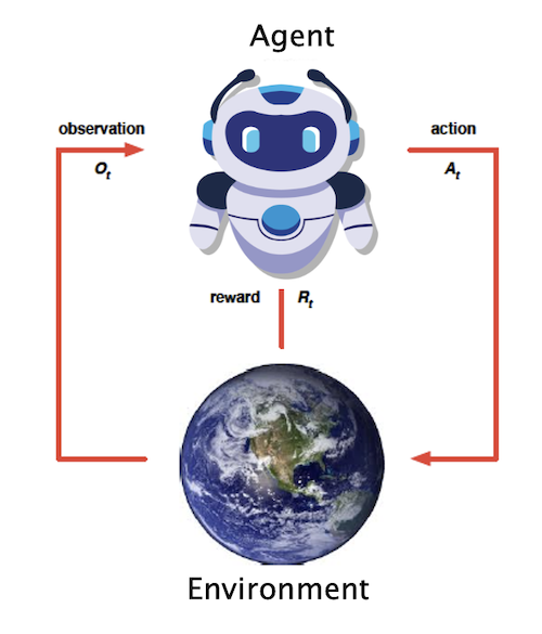
Figure 1: The Reinforcement Learning Control Framework
The easiest way to understand the discipline of RL is to consider how animals, such as dogs, get trained. Since they don’t understand human language, the only way to make them do what we want is by rewarding them when they perform a correct action. Usually this message does not get through to the dog with only a single instance of the reward, but has to be repeated multiple times before the animal makes the association (hence the word ‘reinforcement’ in the name).
A more general picture of the framework used in RL is shown in Fig. 1. There is an agent that is capable of taking one or more actions, and each of these actions results in some change in the environment the agent is operating in. The results of the environment change due to an action are communicated back to the agent as an observation, in addition to a scalar number called the Reward. In order to make the agent carry out a task, which usually takes several actions and thus several traversals though the RL loop, the agent is trained. During the training, if the agent’s actions are such that they make progress towards achieving the objective, then those actions result in a higher reward, and if not then the reward is withheld. Hence the agent gets trained by means of the reward signal, and carries out actions that result in the maximization of the sum of the rewards it receives over the course of the task.
An agent’s actions are a function of its current state, so that A = f(S). The function f is called the Policy Function, and is usually a complex function of the state for cases in which the state corresponds to visual data. In Deep RL this function is modeled as a Neural Network and it is trained using a combination of RL and Deep Learning algorithms.
This technique of using the reward signal as means to make the RL Agent do what we want it to do, works as long as the objective is somewhat simple and of limited scope. However to build agents that are capable to doing more human-like tasks RL, runs into problems. For example if we want to design an robot (controlled by a RL Agent) that is capable of doing our dishes, what reward signal should we use? The basic issue is that the RL Agent does not have an internal model of the world we live in, and also cannot understand language. If you ask a human to do something, how does he (or she) go about the job? We can modify Fig. 1 slightly to show this, as shown in Fig. 2.
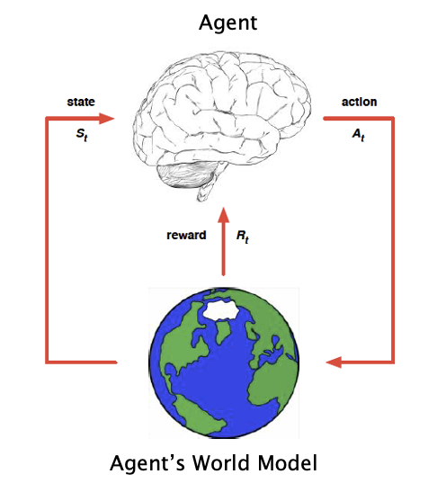
Figure 2: Model Based Control in Reinforcement Learning
Usually the human takes the time to think through, or plan, how to achieve the objective as opposed to immediately starting to take actions. During this planning stage, the human uses a model of the world, to figure out the sequence of actions to take, and the result of these actions will have on the environment. Once the planning is complete, then the task is actually started. The human does not need to be reinforced after each action with a reward, but is able to able to figure out what the sequence of actions to be performed since he understands language and also has a model of the world. Thus, lack of a World Model and lack of language understanding are the two critical shortcomings that have held back RL Agents. Until a few years ago these seemed to be unsurmountable problems. Researchers had little to no understanding of how world models are built in human brains, which is a very complex process that takes place all throughout our childhood and beyond.
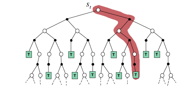
Figure 3: A Decision Tree, with states marked in white circles and actions marked in black dots. The red line shows a path chosen through the tree by an agent
The process of decision making is captured in the graph shown in Fig. 3. The white circles represent the state of the environment, while the black dots represent actions that the agent may take. Note that there is more than one action (black dot) associated with each state (white circle), which models the fact that the agent has a choice of multiple actions that he can perform in each state, and has to decide on the right action. Also once an action is taken, there are multiple possible states that the environment may transition to. This captures the uncertainty in the environment: For example if the agent is playing a video game, then the game may spring an unexpected surprise after the player takes an action. The agent starts the decision making from the top of the graph, and as he performs actions, he proceeds on a path down the graph, until the task is complete (this is shown as a terminal state marked T). Once such complete path is shaded in red in the Fig. 3. Some of these paths result in a successful completion of the task, while others result in failure. While planning how to do the task, the agent has to choose a sequence of actions that result in success.
The Decision Tree shown in Fig. 3 can occur in various different contexts:
- If the task is a problem in Logic or Mathematics, then an action corresponds to a logic or mathematical operation, and the environment is the logical or mathematical model (usually one or more equations in mathematical problems). Hence there is no interaction with the real world and this corresponds to a human solving a problem ‘in his head’.
- If the task involves doing something in the real world, then each action results in some change in the environment. Most applications of Autonomous Agents fall in this category, such as robotics, game playing agents or software agents that interact with the web to carry out some task.
In classical RL, an agent is trained by traversing the decision tree hundreds of thousands of times, until it forms a good mapping from states to actions that maximize the total reward during an episode. An LLM Agent on the other hand can potentially bypass this long training process by using its internal World Model to do task planning, and thus form a plan to traverse the tree and achieve its objective, which is closer to the way that humans carry out tasks.
2.1 Agents of Type 1: Model Free Agents
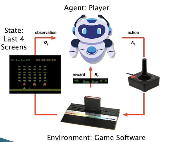
Figure 4: The Reinforcement Learning Framework applied to playing video games
Fig. 4 shows an RL Agent that is being trained to play Video Games. The actions in this case are the movements of the game controller, while the environment or world that the agent operates in, are the successive screens of the game. Every time the agent takes an action, the screen changes and the agent receives a reward from the game. The agent, which is implemented using a Neural Network, is trained by playing the game hundreds of thousands of times, and observing the effects of its actions on the reward and the next screen that is displayed. The RL algorithm used is called DQN which stands for Deep Q-Networks and was discovered by Deep Mind in 2013.
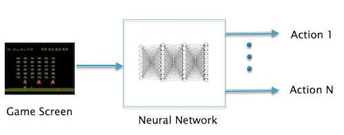
Figure 5: Playing a video game using a Neural Network based Policy Function implementation
Once the agent is trained, it can be used to play the game, and this is shown in Fig. 5. The last few screen shots are fed into the Neural Network, which then predicts what the next action should be. This in turn is fed back into the game which leads to the next screen, which is in turn fed back into the Neural Network, and the cycle continues.
We are calling this type of RL Agent, as an agent of Type 1. These agents are characterized by:
- They are Model Free, i.e., they don’t incorporate a model of the environment they are operating in. Hence the only way to train them is by using Model Free RL, which is a very time consuming process, requiring hundreds and thousands of iterations through the loop shown in Fig. 4. This also means that these agents are incapable of planning in advance. The only way to train them is by dropping them in the real environment in which they will be operating and proceeding by trial and error.
- The policy which they use to take their actions is purely a function of the input state (which in this case is the game screen). This policy is ‘hardwired’ into the Neural Network, so for example, the same agent cannot be used to play other games.
Hence training agents of Type 1 is very much like training a dog, and the trained Neural Network is like the trained dog’s brain, which instinctively knows how to perform the task it was trained for, but not any new task (without further training). This is fundamentally different than the way humans operate, since we are able to plan out our actions in advance using a World Model, which enables us to adapt to new situations we haven’t seen before.’
2.2 Agents of Type 2: Model Based Agents
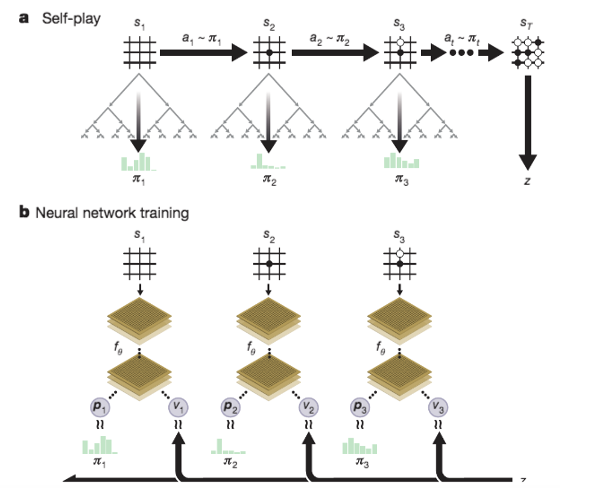
Figure 6a: Illustration of the AlphaZero algorithm from Silver et.al.. Part (a) shows a game being played by using a Decision Tree at each step to find the best move, Part (b) shows a Neural Network being trained to generate the Policy Function and Value Function for the game
There is another type of RL Agent, the most famous example of which the AlphaZero game playing system from Deep Mind. These agents require a model of the game being played, hence its use is limited to board games such as Go or Chess (for these games, a model of the game is the same as the rules of the game). The AlphaZero system incorporates a Neural Network to implement its Policy Function, whose input is the last few board configuration and its output is the next move. This is shown in Part (b) of Fig. 6a where the Neural Network outputs the probabilities p that the Agent should make a particular move. However in addition to the next move, the Neural Network has another output: This is shown as the letter ‘V’ in the figure, and it stands for the probability that the current board position will in fact lead to a winning game. This is analogous to a human looking at the board and making an intuitive judgement whether it will lead to a winning game.
The critical difference between the way AlphaZero plays, vs a Type 1 Agent, is shown in Part (a) of Fig. 6a. Before every move, AlphaZero creates a Decision Tree of possible moves and the corresponding board positions, starting from the current position (this tree is the same as shown in more detail in Fig. 3). This technique is known as a Monte Carlo Tree Search or MCTS (please see Appendix B for a detailed description of MCTS). In order to create the Decision Tree, the agent uses the rules of the game (or model), and also the Neural Network from Part (b) to predict actions. It builds as much of the Decision Tree as it can in the finite time allocated between moves, and from that it chooses the best move to make. Since there is usually not enough time to complete an entire game during tree building process, the winning probability number V used to make an educated guess whether the last board position in the tree is in fact a winning one. Hence the operation of AlphaZero involves a combination of ‘mental planning’ using the Decision Tree, followed by taking an action in the real world of the game. During the planning process, the agent tries out several potential sequences of moves, and then uses this information to choose the best next move. This is closer to the way humans act to achieve an objective, which is a combination of mental planning, followed by actions.
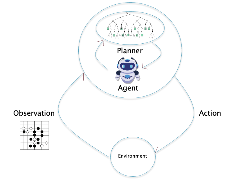
Figure 6b: The Reinforcement Learning Framework for the AlphaZero algorithm
Fig. 6b shows how the original Reinforcement Learning feedback loop from Fig. 4 as modified to reflect the AlphaZero algorithm (the reward signal is assumed to be part of the feedback from the Environment). Whereas a Type 1 agent was ‘pre-trained’ to take actions in response to feedback from the environment without doing any ‘thinking’, with AlphaZero there is an additional Planning Module that the agent invokes to think a few steps ahead before it takes an action. All this planning happens in the agent’s ‘brain’ and does not affect the external environment until the action is actually taken. In order for this to work, the agent needs an internal World Model that is a close approximation to the external environment that the agent is operating in.
The AlphaZero Policy Function module is implemented using a Convolutional Neural Network or CNN, which is trained by having two AlphaZero Agents play against each other. The agent’s policy function is improved during this process by using a type of Policy Improvement algorithm called Policy Gradients. This works by modifying the CNN parameters at the end of each game, as a function of whether the agent won or lost the game.
A major issue with AlphaZero type agents is the fact that they require a model of the environment. Deep Mind later came up with an algorithm called MuZero that is able to play a few board games without knowing the rules of the game. It uses another CNN to build its own model of the game, which is trained as part of the learning process.
Starting in Section 3 we will get into the world of LLM based agents, and we will see that the general learning framework for these agents still fits within the diagram shown in Fig. 6b. The big difference is that the policy function is implemented using an LLM rather than a CNN. Furthermore it has been observed that large pre-trained LLMs such as GPT3 or GPT4 already have model of the world which can be used to generate actions without doing a full RL training of the model. In fact giving the LLM a few examples of the correct policy (called prompting) suffices for it to generate appropriate actions going forward.
The Alpha Zero algorithm is close to a Control Theory technique called Model Predictive Control or MPC, which is widely used for Process Control in Chemical Plants. Just like Alpha Zero, MPC also involves between taking an action in the real world, followed by short horizon optimization using a model of the system being controlled. Only the first step of the resulting plan is implemented, and the cycle continues.
In our daily life, the majority of our decisions are of Type 1 and take place ‘automatically’ or ‘intuitively’ as we go about our day. This corresponds to single pass through our neural network, which has already been pre-trained to do routine tasks through thousands of iterations of training from our childhood onwards. On the other hand, when we perform a task that is not routine, such as planning for a vacation or playing a board game, then it requires planning. This is accomplished by a tree type decision structure shown in Figure 6(a) where various alternatives are fleshed out and weighed for their chances of success. This takes up more of our mental energy, since it requires multiple passes through our neural network. There is an interesting connection between the concepts of Type 1 and Type 2 agents, and the concepts of System 1 and System 2 thinking as proposed by Kahnemann and Tversky. Please see Appendix A for a discussion on this topic.
3.0 LLM Based Agents
Large Language Models or LLMs appeared in 2017 with the system called GPT1 from OpenAI, this was soon after the invention of Transformers, which is the base technology that they use. Since then, OpenAI has released progressively larger models, and the current model is called GPT4 (OpenAI has not revealed the number of parameters in GPT4 but is rumored to be over 1000B). OpenAI also released a version of its LLMs called ChatGPT in 2022, which combined LLM technology with two other techniques: (1) Fine tuning of the LLM using Supervised Learning with human teachers (called Supervised Fine Tuning or SFT), (2) Training of the LLM to avoid toxic and dangerous content as well as hallucinations using a technique called Reinforcement Learning based on Human Feedback (RLHF). The resulting model was released by OpenAI as a service (and also incorporated into the Microsoft Bing search engine), and quickly racked up more than 100 million subscribers within a month of release, faster than any previous technology. This model seems to exhibit an understanding of the world, which it uses to answer questions in a human like manner, and its capabilities far exceed any other LLM that has been released. An especially exciting find is that the model has what are known as Emergent Properties. These are capabilities that have not been explicitly programmed or trained into the model, but the model nevertheless acquires these skills when its size exceeds certain thresholds. Trying to explain how this happens is an active area of research. An important Emergent Properties is the ability to form a model of the environment based on training data and prompts given to the model.
Shortly after the appearance of ChatGPT, researchers began to embed it within the framework of a larger system which they called Autonomous Agents. The motivation behind this was to design more powerful systems that take advantage of the capabilities of the LLM, and also give it additional skills that ChatGPT lacks. These include skills such as: Surfing the Web, using tools such as calculators and WolframAlpha, invoking other Neural Networks for Image Processing or Auditory Processing tasks, synthesis of Python code (which is then executed) etc. Another important addition was that of a memory module, to store the results of intermediate computations.
The common feature of these systems is use of the LLM, not so much for generating text, but as a planner. Given a task, the LLM is able to decompose the work into a series of simpler tasks that it then farms out to itself or to other tools available to it. In order to do this, the LLM needs an understanding of the environment in which the task is to be performed, i.e., it needs a World Model. Evidence has piled in the last year or two that LLMs do indeed form World Models as a result of their training, and this is reviewed in the next section.
3.1 LLMs and World Models
LLMs are trained using Self Supervised Learning on huge corpora of text, by using the next word prediction method. As a result, an LLM in the inference phase works by successively predicting the next word, after it has been given a few words to start off with (called the context). The prediction is done in a probabilistic fashion, with the LLM generating a probability distribution over all the words in the vocabulary, from which a particular word is chosen based on some criteria, such as the word with the highest probability. When LLMs were first invented, over ten years ago, it was thought that the word generation process is purely probabilistic and words are generated on the basis of how frequently the same word occurs in a similar context in the training dataset. However the first LLMs were implemented using less powerful Neural Networks such as RNNs or LSTMs and they were not able to scale up to very large sizes. With the invention of Transformers, it became possible to scale up LLMs to hundreds of millions of parameters, and at the same time train them on massive text datasets. The resulting LLMs, such the GPT3 or the GPT4 seem to have new emergent properties that were not seen in smaller models, and one of these properties seems to be the existence of a World Model. The evidence that is indeed the case has been accumulating, but is not yet universally accepted. For example Yann LeCun has maintained that LLMs are incapable of forming World Models, and he has made the suggestion that visual prediction is necessary for this to happen, which is apparently the way the human brain forms models. The discussion in Section 2.2 shows why the question of World Models in LLMs is so important. If indeed LLMs are forming models of the environment that is used to generate the data they are trained on, then this model can be within the Autonomous Agent context to generate appropriate actions to achieve objectives.
In this section we review the evidence for World Models in LLMs. The first two examples are from the space of Board Games, with Transformers trained not on language, but on sequences of game moves. World Models for Board Games are much simpler than those in the real world, but they are also more tractable due to their simplicity. However they are still complicated enough to enable us to investigate their properties. In the following two Sections we first look at the game of Chess followed by Othello. It is shown that even though the model is trained to predict just the next move, it actually learns to compute the full board state at each move, i.e., the World Model. Hence rather than predicting the next move based on statistical correlations about the distribution of moves, the LLM actually learns to model the underlying process that generated that data.
3.1.1 LLM based World Models in Chess
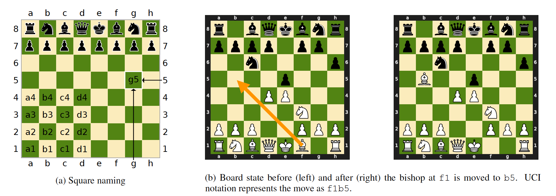
Figure 7: Illustrating the notation used to feed chess moves into an LLM, from Toshniwal et.al.
Traditional LLMs are built using large Transformer models trained with billions of word tokens. Progress is being made in extracting evidence that they indeed incorporate World Models, however another line of research is to look for World Models in simpler systems, such as those encountered in games. World Models for Board Games for example would correspond to the configuration of the board and knowledge of legal moves in the game. It is much easier to look for evidence of World Models within their simpler confines, as opposed to a full scale language model. We review the work by Toshniwal et. al in the context of the game of chess. Transformers can be trained on chess moves instead of word tokens, but otherwise the resulting systems are quite similar.
Tohniwal et.al. point out that even though chess represents a controlled domain, predicting the next move is not a trivial proposition. Consider the board shown on the LHS of Fig. 1(b), where it is white’s turn to move: In order to generate a valid move, the model needs to do the following: (1) Infer that it is white’s turn, (2) Represent the locations all the pieces on the board, (3) Select one of the white pieces which can be legally moved, and (4) Make a legal move of the selected piece. Thus the Transformer model has to learn to track the board state, learn to generate moves according to the rules of chess and also learn chess strategies to predict the actual move.
To program the chess based LLM, Toshniwal et.al. labeled all the positions on the board using a 2D co-ordinate system shown in Fig. 7(a) and then converted chess moves into a linear sequence which is called the Universal Chess Notation (UCI). For example the move shown in Figure 7(b) is represented as f1b5 in UCI, where f1 is the starting position and b5 is the ending position. They converted chess games into a sequence of these kind of moves (for example e2, e4, e7, e5, g1, f3), such that each position corresponds to a single token. They also used a slightly modified version of this system for representing sequences in which only the chess piece to be moved is specified, as opposed to its location (to test whether the model can infer the location of a piece from its name).
These tokens were then fed into the usual Transformer based autoregressive language model, using the standard maximum likelihood objective. The training dataset consisted of 200K games, while the validation and test datasets consisted of 15K games each. Another 50K games were set aside for probing the LLM to detect the presence or absence of a world model. The actual Transformer model used was the GPT2-Small architecture from OpenAI.
The probing of the trained LLM was carried out in two ways:
Ending Square Probing Tasks: The model is given a game prefix and prompted with the starting square of the next move (f1 in the sample in Fig. 1(b)). The model’s next token prediction represents its prediction for the ending square of this move. This probe tests the model’s ability to track the board state (thus deducing the type of piece that is being moved) and follow the rules of chess for that piece, as well as ability to follow strategy.
Starting Square Probing Tasks: In these probes, once again the model is given a game prefix, but prompted with just the piece type for the next move, such as B for bishop. The model’s next token prediction tests its ability to predict where the prompted piece type is located on the board, and thus its ability to track pieces.
Toshniwal et.al. showed that the probes are indeed able to predict the the starting squares and the ending squared with good accuracies (see Tables 5 and 6 in their paper). They also showed that in order to so, the entire game history had to be fed into the model, the performance decreased when only the most recent 50 moves were fed into the model.
We can conclude from this work that the LLM is able to create an internal model of the game state, so that it knows the precise locations of each piece on the board in addition to the allowed legal moves for each of these pieces. It acquires this knowledge entirely from the linear sequence of game moves that were fed into it during the training process. It then uses this information to figure out the identity and position of the piece involved in the next move, as well as the ending position of a piece (given its starting position). This paper makes the case that the LLM is able to do these things by making use of its internal model of the chess board, as opposed to auto regressive statistical prediction of the next move from sequence data being fed into it.
3.1.2 LLM based World Models for the Game of Othello
Inspired by Toshniwal et.al.’s work, Li et.al. observed that the LLMs modeled using chess moves showed the presence of a world model, however the probes used by Toshniwal et.al. did not precisely locate how or where this world model was located within the LLM itself. Li et.al.’s work was undertaken with the objective of addressing this issue, and they did it in the context of the board game called Othello. Othello is a simpler game than chess, but still complex enough so that its moves cannot be predicted by memorization.
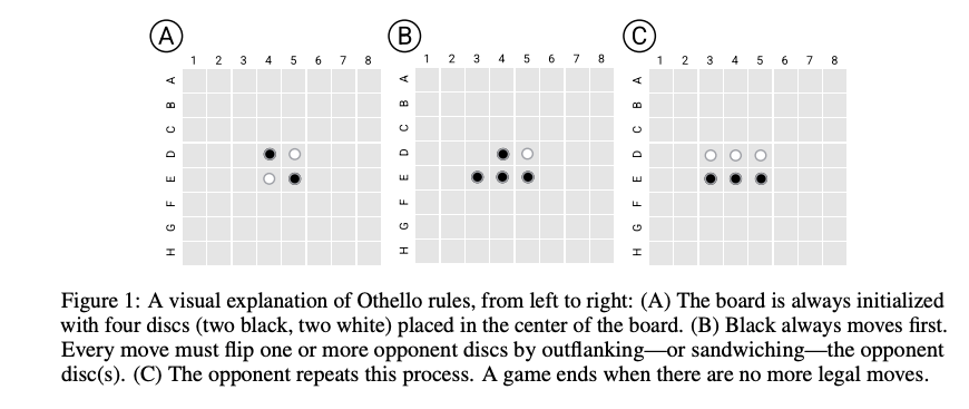
Figure 8: Rules for the game of Othello, from Li. et.al.
The rules of Othello are quite simple and summarized in Fig. 8. There are 64 positions on the board, where the 4 positions in the middle are always occupied at the start of the game, so that there are 60 possible positions that are occupied during the course of the game. Li et.al. trained an 8-layer GPT model with an 8-head attention mechanism and a 512 dimensional hidden space, in an autoregressive fashion, which they called OthelloGPT. This model is fed with a word embedding consisting of 60 vectors, one for each possible board position to get the sequence $(X_1,…,X_{T-1})$, where T is the length of the sequence fed so far. The intermediate activations for the $t^{th}$ token after the $l^{th}$ layer is given by $X_t^l$. Note that $X_{T-1}^8$, which is the last activation vector on the top layer, goes into a linear classifier to predict the logits for the next move.
Li et.al. showed that OthelloGPT was very good at predicting the next legal move, conditioned on the partial games before the move, and this could not be attributed to memorization. Assuming that the model had built an internal representation of the game board, they used a standard tool called a “probe” (see Tenney et.al.), to look for it. A probe is a classifier or regressor whose input consists of internal activations of a network, and output is the feature of interest. If the probe is indeed able to do prediction accurately, then this implies that a representation of the feature is encoded in the network’s activations. For OthelloGPT, the input to the probe was the activations $X_t^l$ for different layers $l$. The output $p_\theta(X_t^l)$ of the probe is a 3-way categorical probability distribution, where the classification is into the states Empty, Black or White. They trained a total of 60 different probes, one for each of the 60 positions on the board. They discovered that linear probes did not work very well, however probes with a single hidden layer were able to predict the board state with approximately 98.3% accuracy. The accuracy was highest for the seventh layer activation $X_t^7$ and decreased to about 95.4% for $X_t^8$. This implies that the model expends its energy in estimating an accurate picture of the board state in the initial 7 layers, and then uses this information in the final layers to do the next move prediction.
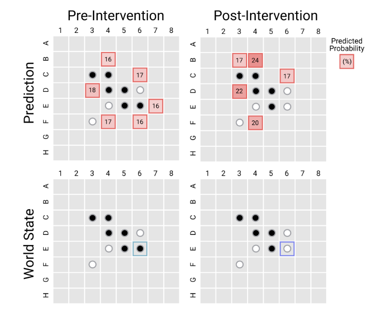
Figure 9: Illustrating that there is a causal relationship between the Board State in the LLM and the next move made by it, from Li. et.al.
So far we have seen that the board state is captured in the activations $X_t^l$ of OthelloGPT. But how can we show that the model is in fact using the information in the board states to make its next move. One way of doing this is by changing the value of $X_t^l$ so that it corresponds to a different board state, and then observing the effect of this change on the next move prediction. This procedure was carried out by Li et.al., and the results on one of the board configurations is shown in Fig. 9. The bottom left figure shows the board state before the intervention, while the bottom right shows the board state after the intervention, the E7 position has been flipped from black to white. The top left figure has the predicted probabilities before the intervention while the top right shows the probabilities after the intervention. As can be seen, the model modifies its predictions to take the post intervention board position into account, which shows a causal connection between OthelloGPT’s board state and its move predictions. The intervention itself is carried out by running the classifier for the position being modified in the backwards direction, and using the error gradients to modify the input $X_t^l$ rather than the classifier parameters.
The examples of World Models that we have presented so far are from the world of games, with the LLM tra ined on the linear sequence of board positions. The next few examples involve LLMs trained on language. These presumably learn a much more complex World Model, and it is interesting to find out their capabilities in this area.
3.1.3 Map Building from Text Prompts
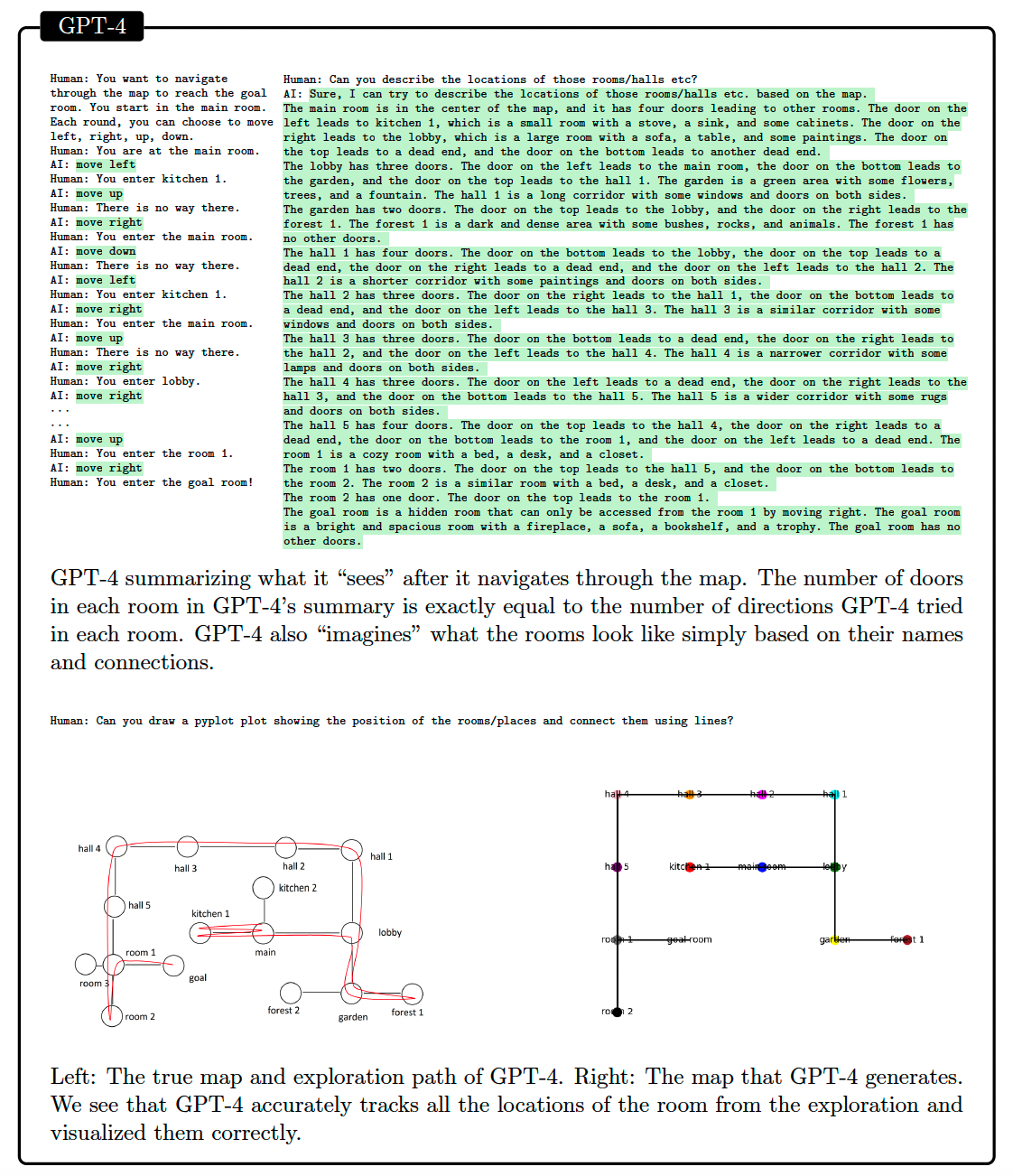
Figure 10: Illustrating that the LLM builds a model of its environment using text prompts, from Bubeck et.al.
We humans build up a mental image of the environment we are in by means of our visual sense. Since the current generation of LLMs don’t have the vision capability, it would be an interesting experiment to find out if an LLM can build a ‘mental map’ of its environment by text prompts alone. Such a map would correspond to a World Model, and can be used by the LLM to do task planning. This experiment was carried out by Bubeck et.al. at Microsoft Research, who used text based games to interact with GPT4. One such experiment is summarized in Fig. 10, in which the LLM is given an objective to navigate through an environment get to a goal. The environment consists of a set of interconnected rooms with doors between them, as shown in the map in the bottom left of the figure. The experiment consists of two parts: In the first part the LLM is prompted with its objective and this followed by a dialogue in which the LLM issues commands to move left, right, up or down and the human responds with a short description of the effect of the carrying out the command (as shown in the upper RHS of Fig. 10). This continues until the LLM reaches it goal room. In the second part of the experiment the experimenters test the ability of the LLM to form a model of all the rooms, by prompting it to describe their locations. GPT4’s response is shown in the RHS of Fig. 10, and is also illustrated in the bottom RHS of the figure. As we can see the LLM’s map of the rooms corresponds to the true map, and the LLM is able to paint an accurate picture of the rooms that it has been in. The response also includes descriptions of the rooms based on what LLM ‘imagines’ them to be, based on their names.
This paper shows that LLMs build an internal map of the world based on the information that is being fed into them. They presumably use this internal map or World Model to formulate their output, as opposed to purely statistical next word prediction. This allows them to handle the ‘covariate shift’ problem i.e., be able to give effective responses to inputs that are not part of their training data. This example of World Model building differs from the prior two, since by using GPT4 we are starting with an LLM that has already been trained. Based on this training, the GPT4 has presumably formed a model for the world, which is why it is able to understand concepts such as ‘left’, ‘right’ or ‘up’, and ‘down’. During the course of the chat session which takes place in the inference mode, GPT4 forms a more specialized World Model that is specific to the information it is being fed during the chat.
3.1.4 Isomorphism between LLM World Models and the Real World
The World Model that LLMs build is obviously of a different nature, than the one that exists in our brains. The latter is based on our sense of vision, sound, touch etc and is grounded in the real world. The World Model in LLMs on the other hand is built entirely on the basis of text sequences, and since LLMs are not embodied and have no sense organs, it is not grounded in the real world. If so, what is the relationship between the LLM’s World Model, and the real world? This question was explored by Patel and Pavlick, who showed that in certain cases the LLM’s World Model is isomorphic (i.e. it has a one-to-one correspondence) to a grounded World Model built by interacting with the real world. This means that the structure of relations between concepts that is learnt by the LLM in text form, is identical to what a grounded model would learn. They carried out their investigation in the areas of Spatial Terms (for example left and right), Cardinal Directions (for example East and West) and RGB Colors.
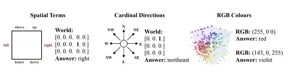
Figure 11: Grounding of the concepts of Spatial Terms, Cardinal Directions and RGB Colors using LLM prompts, from Patel and Pavlick
Fig. 11 shows examples of how the concepts for Spatial Terms, Cardinal Directions and RGB Colors are grounded. In each case the LHS figure shows the grounded concepts, while the RHS has textual representations of the groundings that can serve as prompts for LLMs. In the first two cases the groundings are done using grid world representations, while in the last case it uses 3 dimensional RGB codes associated with the various colors.
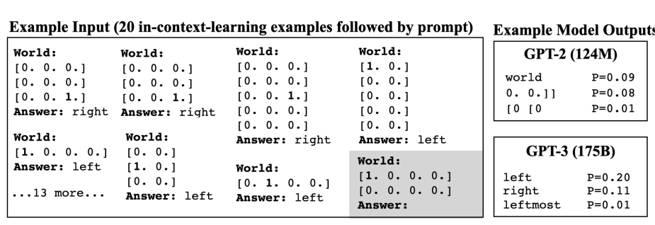
Figure 12: Details of Spatial Terms grounding prompts, from Patel and Pavlick
Fig. 12 shows an example of the grounding process for the Spatial Terms case. As shown in the box on the LHS, a prompt uses the Few-Shot technique and consists of sequence of twenty in-context examples of a grid in which the location of the ‘1’ corresponds to the grounding, followed by the text instantiation of the concept. The last element in the prompt is the question to the model and the two boxes on the right are examples of responses. The top box is for a smaller model called GPT2 with 124M parameters, while the bottom box is for GPT3 with 175B parameters. As we can see the larger model correctly predicts the spatial orientation as ‘left’, while the smaller model is not able to do so. This shows that the model’s ability to form a World Model from its training data is an Emergent Property, i.e., it forms only after the model size exceeds a threshold. This example also shows that the GPT3 model is able to generalize the concept of ‘left’ to ‘unseen worlds’. For example the grid in the final question prompt is different from all the other 20 grids used for in-context learning.
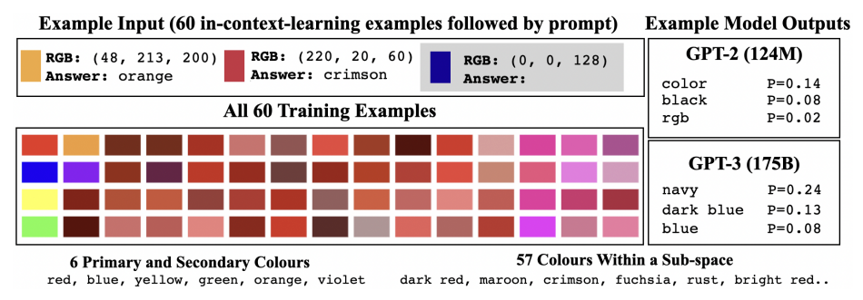
Figure 13: Grounding of unseen colors using partial information, from Patel and Pavlick
Patel and Pavlick also showed the following:
- Generalization to Rotated Worlds: Patel and Pavlick also showed that the concepts of Spatial Orientation and Cardinal Directions also continue to hold in Rotated Worlds. In other words the GPT3 model understands that these are relative concepts, and if the grounding prompt shows a rotated ‘left’ for example, then the ‘right’ is also rotated by the same amount. This also shows that the models are not simply memorizing these concepts.
- Generalization to Unseen Concepts: Instead of grounding the entire conceptual structure to a grounded world, what if we ground only a small subset of points in the domain. Will the model still be able to ground the entire conceptual domain? Patel and Pavlick tested this hypothesis for the Cardinal Directions case, and showed that even if the model was grounded with a subspace consisting of the directions north and east for example, it was still able to identify the directions south and west, even though they didn’t occur in the in-context training examples. They repeated this experiment for the case of Color Grounding as shown in Fig. 13. The grounding was done by using 60 in-context examples of colors which are mostly shades of red, with only a single example of a shade of blue. In spite of this, the GPT3 model was able to correctly identify the shade of blue that it was tested with.
These examples suggest that the GPT3 model has built an internal World Model based on its training examples, so that even if it is grounded on a subset of the world, it is able to use its world model to map to the entire space. In other words it already has the concepts of Spatial Orientations, Cardinal Directions and Colors and has mapped them to an internal representation that it has built. Once a subset of these concepts are mapped in the Grounded World (using prompts), the other points in its internal space also get automatically mapped. In other words the model’s internal World Model is Isomorpic to the Grounded World Model.
4.0 Task Planning Using LLMs
Forming a World Model is only one aspect of how an Intelligent Agent works. The other critical function is to be able to formulate an Action Plan or a Policy, which ultimately results in successful completion of the task assigned to the agent. Using LLMs to formulate a policy is a fast evolving area, with new discoveries and proposals coming almost on a daily basis. In this section we will attempt to survey the current work in this exciting area.
Planning proposals come in two flavors:
-
Decision making with no outside world feedback: In this case the planning happens entirely within the ‘mind’ of the LLM. Thus the LLM relies entirely on its internal World Model to make decisions. Areas such as solving Math Problems or proving Logical Propositions don’t involve external feedback, and are are appropriate for this type of planner. This category of planners can be further divided into single prompt planning and multi prompt planning.
(1) Single Prompt Planners: Algorithms such as Chain of Thought (CoT) and Self Consistency COT (SC-CoT) fall into the category of Single Prompt Planners. These algorithms typically propose a sequence of actions in response to the input prompt, without any mechanism to check whether these actions are in fact useful in accomplishing the goal.
(2) Multi Prompt Planners: Algorithms such as Tree of Thought (ToT) and Reasoning via Planning (RAP) are in the category of Multi Prompt Planners. These algorithms prompt the LLM to propose multiple candidate actions at each step, and then use a mechanism for deciding which of these actions is the best. If a chosen action results in failure to accomplish the task, then the algorithm can backtrack to a previous state and restart the process. The RAP algorithm uses an explicit World Model (also modeled by an LLM) to guide its actions, while in ToT the World Model is implicit.
-
Systems in which Decision Making and Real World Interaction are Interleaved: For this case, also known as Tool Use, feedback from the external world is used to inform the LLMs decisions. This can take several forms: For example, consulting a website or the Wikipedia, robotic manipulation, using a calculator or Mathematica, visual feedback etc. This come with several benefits: (1) The LLM Planner can immediately react to an action that did not work as intended, (2) LLMs sometimes hallucinate their responses, which can be corected with external feedback. Some of the early work in this area, such as the Zero Shot Planner, was of the Single Prompt type, in the sense that the LLM was used to propose a sequence of actions which were then implemented by a Robot. However, all recent work uses Multi Prompt Planners in which feedback from the real world is used to inform the next action. Examples of this include the successor to the Zero Shot Planner called the Inner Monologue system as well the ReAct algorithm.
Towards the end of this section we will show that the most powerful planners are those in which internal planning (with no feedback) is combined with external feedback information to create algorithms that resemble the AlphaGo or MPC techniques.
The Decision Tree diagram shown in Figure 3 and the RL learning loop in Fig. 6b are useful references to keep in mind, since we will see that most planning techniques fit within this framework.
4.1 Single Prompt Planners
4.1.1 Chain of Thought (CoT) and Self Consistency with CoT (SC-CoT)
LLMs were originally prompted by asking them to respond or solve a problem by posing a question as a prompt, with the expectation being that the LLM will complete the prompt with the appropriate answer. This technique worked well for simpler problems, but researchers discovered that if the solution to the problem involved multistep reasoning, then simple prompting did not work very well. Wei et.al. showed that the results could be considerably improved if the LLM was prompted using a prompting technique that they called ‘Chain of Thought’ or CoT prompting.
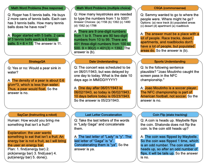
Figure 14: Examples of Chain of Thought (CoT) prompts for arithmetic, commonsense and symbolic reasoning, from Wei et.al.
Examples of CoT prompts are shown in Figure 14 with the CoT in colored highlight (the LLM’s response is not shown), using the format <input, chain of thought, output>, for arithmetic, commonsense and symbolic reasoning benchmarks. As can be seen, the CoT prompt is essentially decomposing the solution to the problem into multiple steps. For example, the CoT for the arithmetic problem in the top left can be decomposed into:
- Initial state $S_0$: Roger has 5 tennis balls
- Action 1: He buys 2 more cans of tennis balls, with 3 balls per can.
- State $S_1$: Since 2 cans hold 6 balls, Roger now has 11 tennis balls.
This decomposition into multiple actions is more explicit in the SayCan robot example in the lower left. Going back to the decision tree shown in Fig. 3, the CoT prompt can be considered to be an example of a successful traversal of the tree, starting from some initial state. By giving the LLM one or more examples of successful traversals, it is able to better replicate the multistep reasoning process involved. Wei et.al. also discovered that the CoT prompting method only works well for the larger models with at least 100B parameters, hence it an emergent property of LLMs.
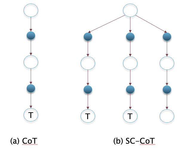
Figure 15: The Decision Trees for CoT and SC-CoT algorithms
The CoT prompting technique can be considered to be a ‘greedy’ method in the sense that it takes a single path through the decision tree to get to its goal, as shown in part (a) of Fig. 15. Wang et.al came up with another prompting technique, which they called CoT with Self Consistency or SC-CoT. The main idea behind this is illustrated in the Decision Tree shown in Part (b) of Fig. 15. Wang et.al. pointed out there are often multiple reasoning paths through the Decision Tree that lead to the same final answer, and one way to make sure that the answer is correct, is by choosing the one that is predicted the most.
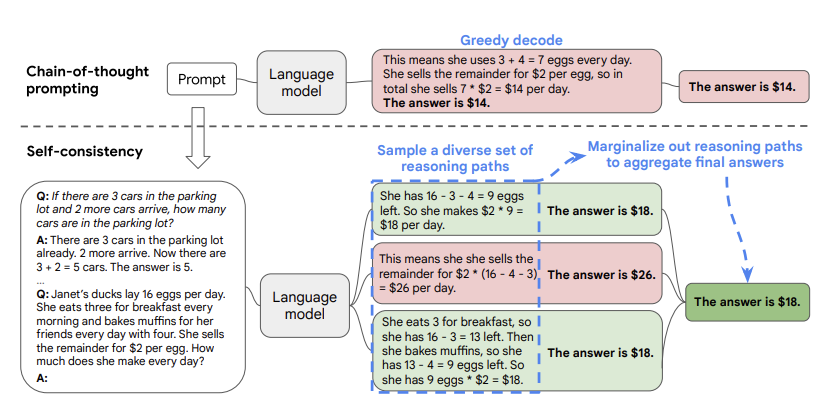
Figure 16: Illustration of the SC-CoT algorithm, from Wang et.al
Figure 16 illustrates the SC-CoT technique. As shown, the prompt is similar to what one would use for CoT prompting. The CoT greedy decoding is shown on the top part of the figure, which results in a wrong answer in this case. The SC-CoT method on the other hand samples multiple times from the LLM, resulting in a different reasoning path each time. Since the $18$ occurs as the final answer on a couple of those paths, it is chosen as the correct result by SC-CoT. Wang et.al. showed that SC-CoT results in a significant improvement in the correctness for complex reasoning tasks compares to CoT, and furthermore has the advantage that it is simple to implement.
The example in Fig. 16 does not cleanly break up the SC-COT flow into States and Actions of the type shown in Fig. 15. For example the top branch in the figure can be decomposed into States and Actions as follows:
- Initial State and Statement of Problem: As shown in the box on the LHS
- Action1: How many eggs does Janet Have?
- State1: She has 16 – 3 – 4 = 9 eggs
- Action2: How much money does she make?
- State 2 (Final): She makes $2*9 = $18 per day
Hence the State in this example corresponds to the current state of the calculation, while the action is the question that triggers the calculation.
Note that the SC-CoT method only works if one of the answers occurs more than 50% of the time. But if the answers are more evenly distributed then this technique will not work. Also a lot of problems posed to the LLM cannot be answered using a numerical value, which also precludes using this method.
Algorithms that are specialized for solving Math problems such as the GSM8K Solver and the MATH solver from OpenAI also fall in the category of Single Prompt Planners, but instead of using a simple majority rule, they use more sophisticated techniques. The GSM8K solver uses a separate LLM fine tuned on detecting the correct solution, to propose a score, and then uses the solution with the highest score. The more powerful MATH solver on the other hand also uses a separate LLM, but now this LLM is used to propose a score for the correctness of each individual step in the solution.
Both the CoT and the SC-CoT techniques are dependent on humans generating good example prompts that can lead to correct reasoning steps by the LLM. Xu et.al. proposed a technique by which the LLM itself can be use to generate the CoT prompt, which they called Reprompting. This requires the use of two LLMs, such that LLM1 is used to generate the example CoT prompts, while LLM2 is used to solve the actual problem. The method works in two steps:
- In Step 1 a number of example CoT prompts are generated by LLM1 by using simple K-shot prompting (this can be done by prompting the LLM to think ‘step-by-step’).
- In Step 2, these prompts are in turn fed back into LLM1 as CoT prompts to further refine them. This results in the final set of CoT prompts that are then used in LLM2 to solve the actual problem (which may be un-related)
4.2 Multi Prompt Planners with Feedback
The CoT method suffers from the following problem: If the solution to the task involves a long chain of thoughts, then an incorrect thought anywhere in the chain can invalidate the final answer. In general LLMs are reasonably good in solving problems that require 2-3 thoughts at most, but stumble on longer chains. The SC-CoT method partially addresses this problem by providing a diversity of chains. However if we examine these algorithms using the Reinforcement Learning framework in Fig. 1, then we see that both these methods generate a series of actions, without incorporating any feedback about the results of those actions on the environment. In this section we will describe a few algorithms that incorporate feedback in order to complete the RL loop. This feedback can take several forms:
- The simplest type of feedback is to decompose the problem in to a series of simpler problems, and then prompt the LLM multiple times to sequentially solve each sub-problem. The response to a sub-problem is fed back into the LLM to facilitate the answer to the next sub-problem. The Least-To-Most Prompting algorithm was one of the first to use this technique.
- A more comprehensive feedback can be provided by using a second LLM which is specialized for this task. For example the Self-Correction algorithm uses the second LLM to provide feedback in the form of a scalar value after each LLM generated action, which is added to the subsequent prompt. The REFINER algorithm has a similar design, with the second LLM providing a more detailed verbal feedback after each action. Both these algorithms use fine tuning of the second LLM in order to train it to give the appropriate feedback.
- Instead of following a linear sequence of prompts followed by actions, the RAP and the ToT algorithms use a multi-branched Decision Tree structure instead. Hence the LLM proposes more than one action at each step, and one or more of these actions is chosen to continue the process. RAP proposes to use the MCTS algorithm to navigate the tree to find the best decision making sequence, while ToT uses the Depth First Search or the Breadth First Search technique. In both the cases rewards are assigned by using a second LLM. RAP also uses another LLM to predict the next state in response to an action, while ToT simply feeds back the result of the action as the feedback. Both these techniques allow the decision making to fall back to a previous node in the tree in case of task failure (as opposed to restarting from the root node).
4.2.1 Least-to-Most Prompting and REFINER Algorithms
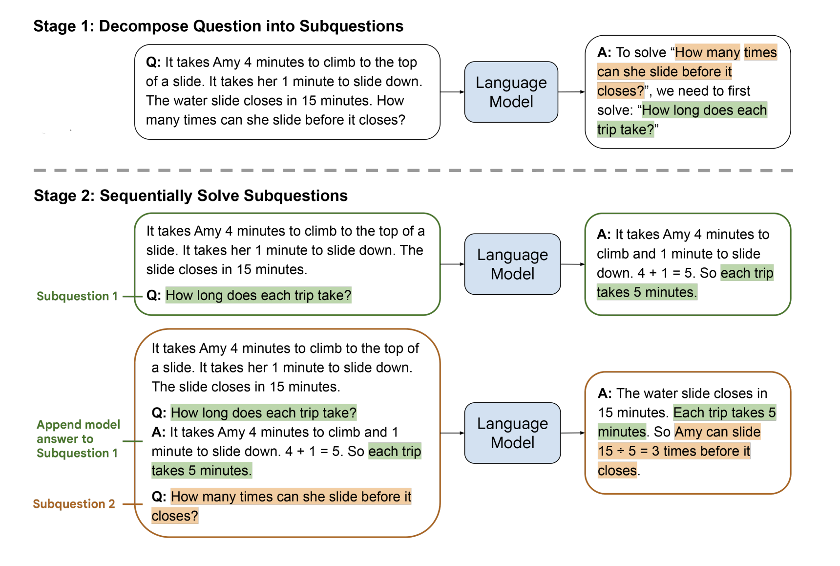
Figure 17: Illustration of the Least-to-Most prompting algorithm, from Zhou et.al.
The Least-to-Most prompting algorithm is illustrated in the Fig. 17. In Step 1 The LLM is prompted with examples of how to decompose a problem and solve it in stages (this prompt is not shown in the figure). In Step 2 the LLM is prompted to solve the problem, by using the decomposition in Step 1. As shown in the example in the figure, the LLM decomposes the problem into the sub-problem “How long does each trip take?” in Step 1. In Step 2 the LLM solves this sub-problem and the solution is fed back along with the original problem into the LLM, which then generates the final answer. This technique can be combined with SC-CoT to further improve performance.
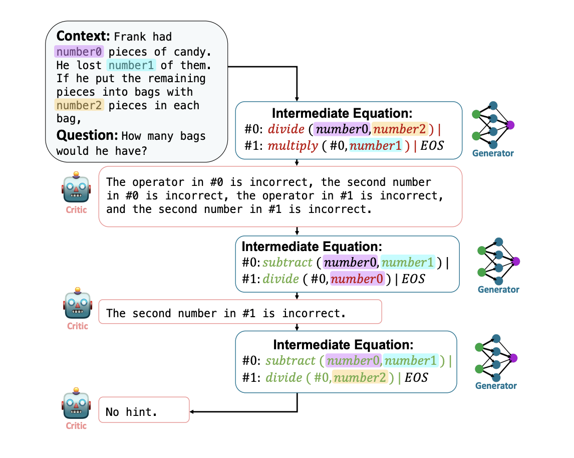
Figure 18: Illustrating the Critic and Generator LLMs in the REFINER algorithm, from Paul et.al.](https://arxiv.org/pdf/2304.01904.pdf)
The Least-to-Most technique certainly helps by decomposing a problem into a sequence of simpler sub-problems, but if any of the intermediate steps are in error, then it nullifies the entire chain. Several researchers have come up with ways to mitigate this issue. A possible solution is to provide a scalar score as feedback to each step. However in natural language reasoning problems defining such a scalar value is not straightforward. Paul et.al. proposed an alternative feedback technique called REFINER whereby a second LLM is used to give verbal feedback. This LLM is referred to as the Critic and is explicitly trained to do this task, while the main LLM generating the responses is called the Generator. [Paul et.al.] showed that the Critic LLM can be a much smaller model than the Generator LLM, while still being able to provide good feedback. The Generator and the Critic models interact with each other during the process of solving the problem, as shown in the Fig. 18. Also the Generator and the Critic are fine tuned together during the training process.
4.2.2 The Reasoning via Planning (RAP) and Tree of Thought (ToT) Algorithms
In this section we describe a couple of methods, referred to as Tree of Thought type methods, that can potentially improve performance. They are characterized by the following:
- The Decision Tree now resembles the tree shown in Fig. 3. Hence instead of a single chain, these algorithms can potentially branch out from any of the nodes in the tree.
- The decision making LLM is prompted multiple times during the course of the tree traversal, as opposed to just once at the root node as in CoT or SC-CoT. Hence after each prompt, the LLM has to make only a few decisions, which improves the chances of success.
- The methods come with techniques to evaluate the quality of the decision being made, based on which they can backtrack to an earlier node to recover from errors.
We will describe two algorithms that fall into this category, called Reasoning via Planning or RAP and Tree of Thought or ToT. The RAP algorithm follows the Reinforcement Learning formulation with its explicit separation of Decision Tree nodes into Action Nodes and State Nodes. It also uses two LLMs such that LLM1 is used to make decisions, while LLM2 is used to update the state of the system. Furthermore it uses the Monte Caro Tree Search (MCTS) algorithm to traverse the tree (see Appendix B for a short description of MCTS). The ToT algorithm on the other hand adopts the CoT design in which action nodes and state nodes are one and the same. Both these algorithms proceed by prompting the LLMs multiple times during the course of the tree traversal.
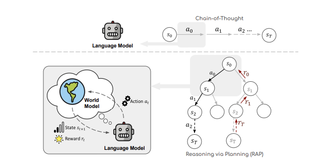
Figure 19: Overview of the RAP framework, from Hao et.al.
Hao et.al. adapted MCTS to work with LLMs and came up with an algorithm they called Reasoning via Planning (RAP). A high level view of RAP is shown in Fig. 19. As shown, it adopts the usual Reinforcement Learning framework for decision making, with the caveat that LLMs are used to propose appropriate actions, as well as for keeping track of the current state. This framework adopts two LLMs for its functioning, with LLM1 (called the Action LLM) used to propose actions while LLM2 (called the State LLM) is used to keep track of the current state. This is a point of differentiation from CoT or SC-CoT, since in those systems a single LLM keeps track of both the action and state which are mixed together. Note that the Action LLM is sampled multiple times in RAP in order to generate the multiple actions after each state.
The graph shown on the RHS of the figure is referred to as a Markov Decision Process or MDP in Reinforcement Learning nomenclature. It consists of the tuple $(S_t, A_t, R_t, p), t = 0, 1, …, T$, such that the action $A_t$ at time step $t$ is distributed according to $p(A\vert S_t,c)$ where $c$ is a prompt used to steer the LLM for action generation, the state $S_{t+1}$ is distributed according to $p(s\vert S_t, A_t, c’)$ where $c’$ is another prompt used to guide the LLM to generate the next state. The Markov in the name refers to the fact that both the Action $A_t$ and State $S_{t+1}$ are entirely determined by the prior State $S_t$, and are independent of what happened before.
An important decision point in applying the MCTS algorithm to LLM based Decision Trees is the allocation of rewards in the MDP. Hao et.al. proposed the following ways in which the reward could be allocated:
- By using the Likelihood of the Action: This can be computed as the log probability of the action, where the probability of the action can be computed using the Action LLM output.
- Confidence in the state that results from taking the action: This can be done by drawing multiple answers from the State LLM and using proportion of the most frequent answer as the confidence level.
- Self-Evaluation by the LLM: This can be done by appropriately prompting the Action LLM.
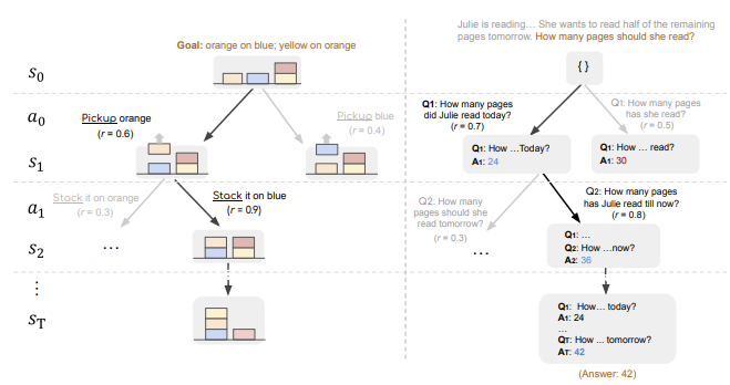
Figure 20: Example applications of RAP, from Hao et.al.
Fig. 20 has two examples of how state and actions can be chosen to solve problems using LLMs. The example on the left consists of a set of colored blocks arranged in a starting configuration, with the goal of the problem being to re-arrange the blocks in a particular fashion. In this case the system state corresponds to the current block configuration, while an action is picking up and placing blocks. The example on the right shows how RAP can be used to solve Math problems. In this case the state corresponds to the current state of the calculation, while actions correspond to questions posed by the LLM to move the solution along. Note that in both these examples the Decision Tree is generated without interacting with the real world, i.e., it corresponds to a human contemplating how to do a task. In contrast to CoT, states and actions are explicitly separated out into their own nodes in the Decision Tree. This allows multiple actions to be associated with each state (or multiple states to be associated with the same action), thus creating the tree structure. This is made possible by the fact that two separate LLMs are used to generate actions and states respectively.
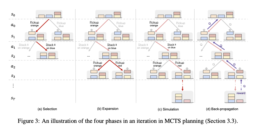
Figure 21: Illustration of MCTS planning, from Hao et.al.
Fig. 21 shows how RAP uses MCTS to solve the BlockWorld problem. It shows the four stages of MCTS, i.e., Selection, Expansion, Simulation and Back Propagation, and it closely follows the general MCTS description given in Appendix B. During the Selection Phase the UCT algorithm (which stands for Upper Confidence Bound Applied to Trees, see Appendix B for a definition) is used to choose the child nodes in the part of the tree that has been fully built out. Once the tree traversal reaches one of the leaf nodes, the Expansion phase kicks in, during which $d$ action nodes are added by LLM1, followed by the addition of $d$ corresponding state nodes by LLM2. From these $d$ nodes, the node with the largest local reward is picked for the next phase. During the Simulation Phase the algorithm successively adds actions and states until the Terminal State is reached. Once again actions with the highest local reward are chosen during this phase. The Back Propagation Phase involves the calculation of the $Q(s,a))$ values for the decision tree using the formula given in Appendix B.
Once a pre-determined number of MCTS iterations is reached, the algorithm stops the tree building process, and proceeds to chosse the best path through the tree using some criterion. Typical criteria include choosing the path with the highest Q values, or choosing the path with nodes that were vistited the most etc.
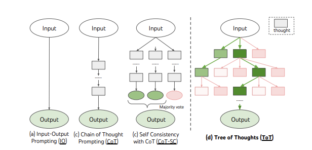
Figure 22: The ToT algorithm and its comparison with IO, CoT and SC-CoT algorithms, from Yao et.al.
Yao et.al. presented another tree based Planning Algorithm that they called Tree of Thoughts or ToT. The main idea behind this algorithm is illustrated in Fig. 22, and is also contrasted with the CoT and the SC-CoT algorithms. This algorithm does not cleanly break up the Decision Tree into state and action nodes like the RAP algorithm, it is more of a tree extension to the CoT or SC-CoT algorithm as explained below.
Using the notation $p_\theta$ to denote a pre-trained LLM with parameters $\theta$, and lowercase letter $x,y,z,s,…$ to denote a language sequence so that $x = (x[1],…,x[n])$ where each $x[i]$ is a token, it follows that $p_\theta = \prod_{i=1}^n p_\theta(x[i]\vert x[1,…,i-1])$. Input-Output Prompting with the prompt sequence $IO$ and using $x$ to generate $y$ such that $y$ is distributed according to $p_\theta(y\vert prompt_{IO}(x))$, and for simplicity this is shown as $p_\theta^{IO}(y\vert x)$. Using this notation CoT prompting can be represented as follows: Given input $x$ and output $y$, let $z_1,…,z_n$ be the chain of thoughts that result in $y$ given $x$. CoT works by sampling each thought $z_i$ distributed as per $p_\theta^{CoT}(z_i\vert x,z[1,…i-1])$ sequentially followed by the output $y$ which is distributed according to $p_\theta^{CoT}(y\vert x,z[1,…,n])$.
Each state in the ToT algorithm is represented as $s = [x,z[1,…i]]$ in this notation, starting with the Root State $x$, and then adding the thoughts as we descend the tree. Note that this is a different definition of state as compared to the RAP algorithm, since in the latter case the state corresponded go the state of the environment and was generated by a second LLM, while for ToT the state tracks the current state of the sequence of thoughts $z$. Since ToT is a tree model, multiple new thoughts have to be generated from state $s$, and the most straightforward to do this is by sequentially sampling i.i.d. thoughts using CoT prompting, one after the other.
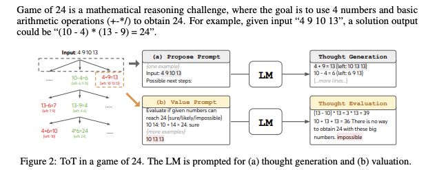
Figure 23: ToT appied to the game of 24, from Yao et.al.
If there are multiple states to choose from, then which should be used in proceeding down the tree? [Yao et.al.] proposed a couple of ways to evaluate states: (1) Use the same LLM to generate a Value $v$ for each state, using the Value prompt $V(p_\theta, S)$ which is distributed according to $p_\theta^{value}(v\vert s)$. $v$ can be either a number say $1,…,10$ or a qualitative word such as (Sure,likely,impossible). (2) By using the LLM to Vote across all the candidate states. This is illustrated in Fig. 23, where the LLM is used to play the Game of 24, where the goal is to use the 4 numbers and basic arithmetic to obtain the number 24. Starting from the root node, the LLM makes multiple proposals, and the figure shows how the proposal in the right branch of the tree is evaluated.
The final missing piece in the ToT algorithm is the method to be used in traversing through the tree. [Yao et.al.] proposed Breadth First Search (BFS) or Depth First Search (DFS) as ways in which this can be done. BFS works by maintaining a set of the $b$ most promising states per step, while DFS works by choosing the most promising state first until the final output is reached or the State Evaluator decides that it is impossible the solve the problem from the current state $s$. If the latter happens then the subtree from $s$ is pruned and the DFS backtracks to the parent state of $s$ to continue exploration.
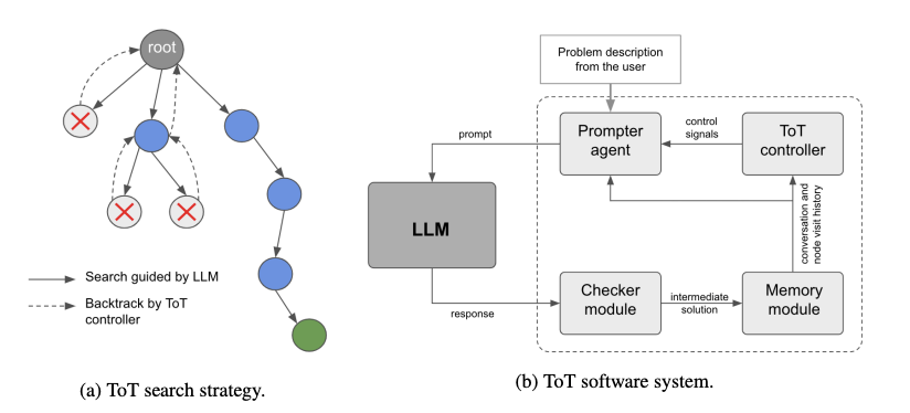
Figure 24: Software architecture to support Tree of Thought type algorithms, from Long
These tree based techniques require a surrounding software infrastructure to do things like putting together multiple prompts during the course of the tree traversal, integrating the operation of multiple LLMs, storing intermediate results in a memory module etc. A possible architecture for doing this is shown in Fig. 24, and is from the paper by Long. This paper proposes a Tree of Thought algorithm is similar to the ToT algorithm described earlier.
4.2.3 The Problems of Tree Traversal and Reward Allocation
Tree based Planning Algorithms such as RAP and ToT have less than optimal ways for doing tree traversals. In the case of RAP the best action is chosen as the one that has the highest log probability as computed by the LLM. This method is a bit suspect since the reward should be determined not by the action but the consequences of the action on the environment, i.e., it should take the resulting state into account as well. Both these algorithms use the technique of prompting the LLM itself to suggest the best way to proceed which may work better if the LLM has a good grasp of the task objective and the current state of the environment. These techniques can be characterized as ‘greedy’ decision making in the sense that the choice is made on the basis of the immediate reward. Reinforcement Learning teaches us that the best decisions are taken on the basis of long term rewards, i.e., an action that leads to short term pain can result in long term success. RL accomplishes this by making decisions not on the basis of highest reward for the next step, but by keep track of long term rewards in the form of the Value Function $Q(S,A)$, and then choosing the action that has the highest Q value.
A related problem is that of verifying the correctness of the final solution. Just choosing the solution that occurs the majority of times does not always work, as was pointed out in Section 4.1.1.
Cobbe et.al. and Lightman et.al. from OpenAI proposed another solution to the verification problem, namely by training a separate Verification Model. These methods have been applied to the SC-CoT type algorithms in Math datasets. [Cobbe et.al.] trained and tested their system on the GSM8K dataset, while [Lightman et.al] used the more difficult MATH dataset.
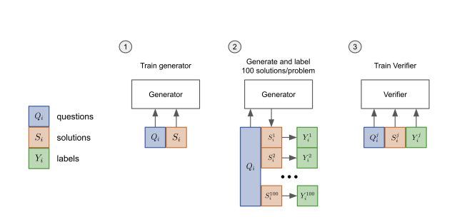
Figure 25: Illustration of Generator LLM and Verifier LLM training, from Cobbe et.al.
The proposal by [Cobbe et.al.] is illustrated in the Fig. 25 and works as follows:
- The LLM model that generates the solution is called the Generator. In Step 1 it is fine tuned using Ground Truth solutions to the problems for a total of two epochs. The Fine Tuning is done by having the Generator generate 100 possible solutions to each of the problems, and then by running each of those (Question, Answer) pairs through the Generator, and comparing the generated answer with the correct solution.
- In Step 2 the fine tuned Generator is used to generate another 100 solutions, and each of those solutions is labeled as correct or in-correct by a human labeler.
- In Step 3 a separate LLM is trained as a Verifier for a single epoch by inputting it with a Question, followed by the Answer and then the correct Label. The output of the Verifier is the probability that the solution is correct. In addition the Verifier is also trained with the same language modeling objectives as the Generator.
In the Inference mode, the Generator is used to sample 100 solutions to a problem, these are then ranked by the Verifier and the solution with the highest score is returned. Since the Verifier ranks only the final output, this method is called Output Supervised Reward Model of ORM.
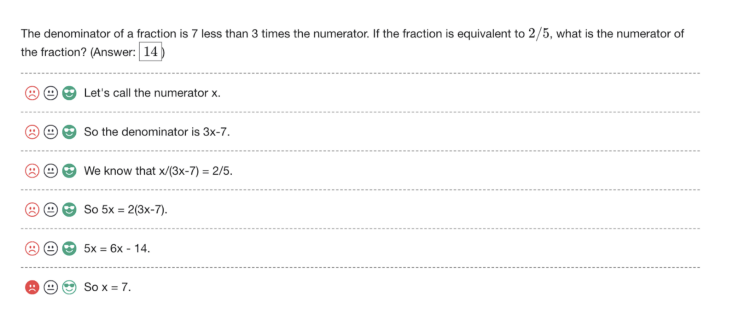
Figure 26: An example of labeling in the PRM method, from Lightman et.al.
The Verifier LLM in the paper by [Cobbe et.al.] was trained by assigning a single correct/incorrect label to a prospective solution. [Lightman et.al.] showed that the performance of the Verifier could be improved if the verification is done on a step-by-step basis instead, which is called Process Supervised Reward Model or PRM. An example of how labeling can be done for this case is shown in the Fig. 26. Each step of the solution is labeled with one of three choices: Positive, Negative or Neutral. Positive indicates that the step is correct and reasonable, Negative indicates that step is either incorrect or or unreasonable, while the Neutral label indicates ambiguity. During inference Neutral labels are treated either as Positive or Negative. Under this system, the score for a complete solution is defined to be the probability that every step is correct, and is computed as the product of the corectness probabilities for each step. Note that step-by-step verification also comes with the following benefit: In case the solution is in-correct, the Verifier is also able to identify the exact step at which the error occurred.
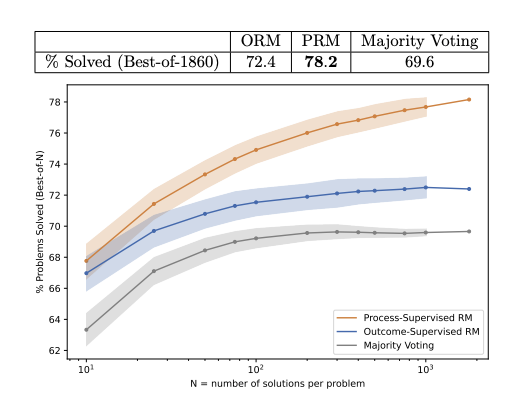
Figure 27: Comparison of the ORM, PRM and the Majority Voting methods, from Lightman et.al.
The ORM, PRM and the simple-majority rule used in SC-CoT are compared in the Fig. 27. The y-axis is the percentage of problems that were solved correctly, while the x-axis is the the number of solutions N that were generated for each problem. Note that ORM performs slightly better than the majority voting baseline, while PRM strongly outperforms both, and the performance gap widens as N increases. From this [Lightman et.al.] concluded that PRM is more effective than both ORM and majority voting at searching over a large number of model generated solutions.
It is conceivable that a modified version of the PRM method can be applied to tree based algorithms such as RAP or ToT. If so, the choice of action can be based on the rewards being generated by the PRM model as opposed to those being supplied by the main LLM model being used to generate the actions. Since the PRM model probabilities are grounded on fine tuning provided by humans, we can expect them to be more accurate. However this requires that the modeler have access the source LLM model for fine tuning.
4.3 Multi Prompt Planners with Interleaving of Planning and Environmental Feedback
The Planning Algorithms described in the previous section don’t involve any interaction with the real world environment the agent is operating in. This is sufficient for applications such as solving Math problems or Logical Puzzles, however there is an important class of problems in which the plan that is produced has to be implemented in the real world. Applications such as robotics or using the system for interacting with software applications such as web searching or other tools fall in this category. In these use cases the LLM has access to the state of the real world, and after every step of the Decision Tree it can get feedback on the effect its actions are having on the world around it. However it still needs its own internal model of the world to do its planning, which can follow one of the planning methods described in the Section 4.2.
One of the first applications which showed the feasability of using LLMs in Robotics was by Huang, Abbeel et.al.. Their work can be considered analagous to ToT in the sense that the LLM is used to generate a chain of robotic actions in response to a series of prompts. However these prompts don’t contain any feedback from the environment or an internal World Model. This was improved upon by the Inner Monologue (IM) algorithm proposed by Huang, Xia et.al. who showed that by incorporating environment feedback and also feedback on whether an action was successful (or not) led to a much improved system. In both these systems the actions proposed by the LLM were translated into manipulations that the robot could actually carry out by using a nearest neighbor type mapping technique. The REACT algorithm that was proposed recently by Yao et.al. can be seen as a further generalization of IM with the incorporation of LLM generated commentary on its own progress, which was added to the state of the system.
In case the chain of actions taken by the agent results in failure, all the three algorithms react by re-starting the process from scratch and trying multiple times until success is achieved (or some retry threshold is reached), i.e., they are not able to learn from the failure to try improving their policy. The Reflexion algorithm proposed recently by Shinn et.al. rectifies this to some extent by having the LLM Agent ‘reflect’ on causes of failure for unsuccessful decision chains. This information is then stored in a long term memory, which is utilized by the LLM to improve its performance in subsequent tries.
4.3.1 Using LLMs for Planning in Robotics: The Zero Shot Planning and Internal Monologue (IM) Algorithms
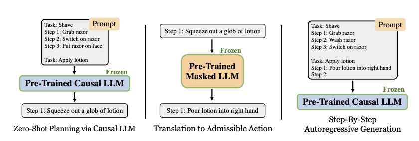
Figure 28: Generation of prompts in the Zero Shot Planning algorithm, from Huang, Abbeel et.al.
Huang, Abbeel et.al. showed that pre-trained LLMs that were large enough, had the ability to decompose high level tasks given to robots into mid-level plans, without further training (with proper prompting). The actions recommended in these plans were further mapped to low level tasks that the robot was actually capable of executing. An example of this is shown in Fig. 28. The LHS shows how the robot was prompted to perform the task “Apply Lotion”, this was done by prompting it with the actions required to perform a similar task of shaving. This resulted in the LLM recommending the action “Squeeze out glob of lotion” as the first action. However this action could not be implemented by the robot since it did not fall within its repertoire of Admissible Actions. The middle part of the figure shows that the recommended action is fed into another LLM that maps it to an Admissible Action that is closest to it. This is done by using Cosine Similarity using the formula
\[C(f({\hat a}), f(a_e)) = {f({\hat a})\cdot f(a_e)\over{\vert\vert f({\hat a})\vert\vert\ \vert\vert f(a_e)\vert\vert}}\]where $f$ is an embedding function that was implemented using a BERT model, ${\hat a}$ is the LLM predicted Action and $a_e$ is the Admissible Action. The RHS side of the figure shows that the generation of the next Action by the LLM is done by feeding the Admissible Action as part of the next prompt, which results in a step-by-step autoregressive generation of the next action. Furthermore the design also included the idea of sampling multiple actions at each step, and then choosing the action that has the maximum mean log probability. Thus this can be seen as an earlier example of the Tree of Thought (ToT) algorithm, using the Depth First Search method to navigate the Decision Tree (the actual criteria to choose the best action takes into account both the mean log probability and the cosine similarity values, as shown in Equation (3) of the paper). However, unlike ToT, this algorithm did not allow for backtracking to an earlier State in the tree in case of failure. [Huang, Abbeel et.al] also showed that the ability to generate realistic plans was an Emergent Property of LLMs, such that the smaller models such as GPT2 not performing as well as the 175B model GPT3.
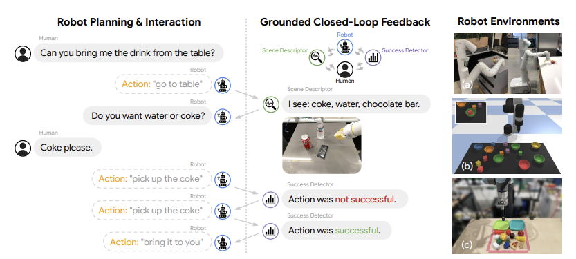
Figure 29: Operation of the Inner Monologue algorithm, from Huang, Xia et.al.
A problem with the [Huang, Abbeel et.al.] algorithm is that fact that it does not allow for any feedback from the external environment. This was rectified by Huang, Xia et.al with an algorithm that they called Inner Monologue (IM). This algorithm closed the Reinforcement Learning feedback loop shown in Fig. 4, by enabling the environment to provide feedback, potentially after each action. This feedback or IM is always in the form of text and can take the following forms:
- Success Detection: This provides the robot with the information whether its action succeeded. If not, then the robot goes ahead and repeats it last action. The Success Detector can be implemented by another Neural Network which has been trained to detect success or failure.
- Passive Scene Description: This is used to describe objects that are visible to the Robot, and can be implemented using a Convolutional Neural Network that does Object Detection and Recognition.
- Passive Scene Description: This allows the LLM to directly ask questions to which answers are provided. This can be implemented either by a person, or by a Visual Question Answering Neural Network.
An example of the operation of this system is shown in Fig. 29, where the Robot is tasked with picking up a can of Coke and bringing it to the Human. The LHS of the figure shows the actions proposed by the LLM, while the center part shows the feedback from the environment after each action. [Huang, Xia, et.al.] also observed that the LLM can respond to human interventions, and can even change the the high-level goal mid-task. It also exhibited interactive understanding of the scene based on past actions and environmental feedback.
4.3.2 The ReAct Algorithm: Combining Reasoning with Acting
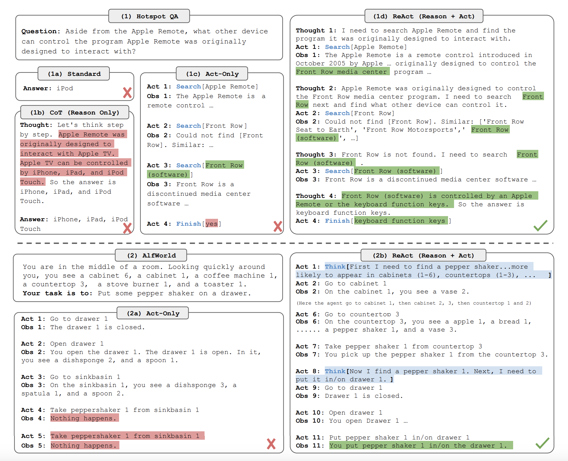
Figure 30: Illustration of the ReAct algorithm for the Hotspot QA and AlfWorld applications, from Yao et.al.
Yao et.al. pointed out that the IM algorithm took environmental feedback such as the scene description or success/failure into account, but did not do what they called ‘verbal reasoning’ regarding the problem being solved. They proposed that adding this new component can lead to an increase in success rate for the agent. Fig. 30 shows an example of how ReAct differs from previous methods. Part (1) is the task posed to the Agent, (1a) is just standard prompt completion while (1b) is the (incorrect) answer proposed by the CoT method which doesn’t incorporate feedback from the environment. Part (1c) shows the response to this problem by an Agent using the IM type algorithm that does get feedback regarding its actions, but is not able figure out the cause of failure. Part 1(d) shows how the ReAct algorithm would solve the problem, and is characterized the following:
- There is an initial Thought at the start of the process that lays out a plan of action on how to go about solving the problem.
- Interleaving of Thoughts and Actions: Every action is followed by an observation (or environment feedback), and this followed by a Thought. A Thought is just the LLM reasoning about the feedback that was just received and planning out its next action.
In order to get the process started, the LLM is prompted initially by a prompt with a few-shot in context examples, which have both domain specific actions as well as free-form language thoughts for task solving. Thus each in-context example is a human trajectory of actions, thoughts and environment observations to solve a task. [Yao et.al.] point out that a strict interleaving of thoughts and actions is only necessary in reasoning dense tasks, while some tasks require the thought module to be invoked less frequently, and this decision is left up to the LLM. In comparison to other planning methods, the paper shows that ReAct always performs better than the CoT method, since the latter is subject to hallucinations due to lack to real world feedback. However the SC-CoT method is quite competitive with ReAct, and in fact does better than it in some cases. [Yao et.al.] attribute this to the fact that ReAct often gets stuck in a error pattern in which the model repetitively generates the previous thoughts and actions. Perhaps this failure mode can be avoided by having ReAct adopt a tree based Planning method such as ToT, such that if the number of repetitions increases beyond a threshold, the the algorithm can backtrack to a previous node and try out some other action.
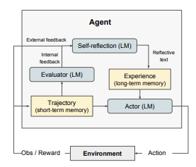
Figure 31: The Reflexion algorithm, from Shinn et.al.
Sometimes an LLM planner is not able to successfully perform the task given to it. When this happens, how can we ensure that the LLMs policy improves from episode to episode, so that it is able to learn from past failures and improve its policy. Shinn et.al. proposed an algorithm called Reflexion to enable a Policy Improvement like behaviours in LLM Agents without the use of Policy Gradients. The operation of this algorithm is illustrated in Fig. 31 and is as follows: The Actor module is implemented using the ReAct algorithm and is responsible for taking the actions as before. After an episode is complete, it is stored in a Short Term Memory module called Trajectory and is evaluated using an Evaluator Model. This module assesses the quality of the generated trajectory by computing a Reward score that reflects its performance. It is not straightforward to do so, and depends on the type of task. The Self-Reflection module, which is implemented as an LLM, plays a crucial role by generating verbal self reflections to provide feedback for future episodes, which is more informative than scalar Rewards. This is then stored in the Long Term Memory module and can be accessed by the Actor for generating future trajectories. Shinn et.al applied the Reflexion algorithm to Sequential Decision Making, Reasoning and Programming tasks and observed improvements over using the plain ReAct agent.
5.0 A Proposal for an Improved Autonomous Agent Algorithm
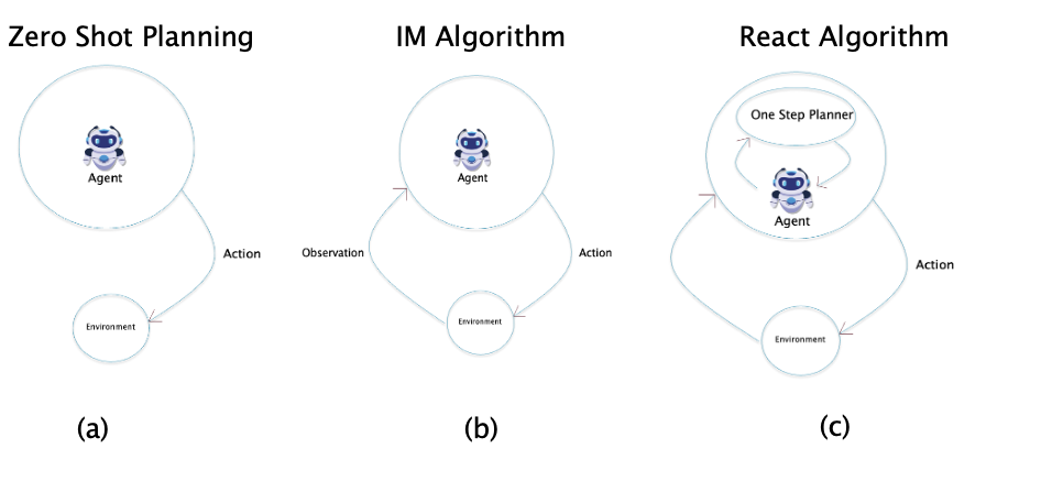
Figure 32: Comparison of LLM planning algorithms
Fig. 32 illustrates the three types of algorithms we have discussed in Sections 4.3.1 and 4.3.2 with the help of a Reinforcement Learning type feedback loop. Part (a) of the figure shows the Zero Shot Planning Algorithm in which the LLM proposes a series of actions which are then carried out by the robot with no feedback from the environment (with the caveat that only actions that can be mapped to those allowed by the robot are allowed). Part (b) of the figure shows the IM algorithm, which falls squarely in the regime of traditional RL algorithms, with the LLM serving as the Policy Function for generating actions and with other Neural Networks providing environmental feedback. Part (c) of the figure shows the ReAct algorithm, which adds an internal Planning (or Reasoning) Module to the system. However the Planning Module is a simple one step type planner, with no ability to be able to retract to a prior node in case of failure.
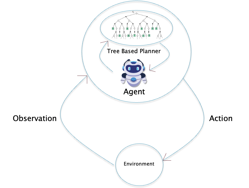
Figure 33: The proposed MPCL algorithm
Fig. 33 shows a proposed algorithm which builds on ReAct, called MPCL (short for Model Predictive Control using LLMs). It is characterized by the following:
- Just as in ReAct there is an LLM (say LLM1) based Planning Module, however it is now based on tree type planner of the type we saw in the RAP and ToT algorithms (see Section 4.2.2). This planner is invoked at the start of the cycle, and also after each environmental feedback.
- At each invocation of the planner, the module builds a decision tree while starting from the current state of the environment. This tree does not extend all the way to the end of the task, but is built to a depth of k, where k is an adjustable parameter.
- The planner uses a separate LLM (say LLM2) to track the state of the environment and this information is used to build the decision tree in a manner similar to the RAP algorithm. This model is constantly updated in response to environmental feedback.
- Based on the information in the decision tree, the agent chooses its next action. This choice can be done using the MCTS algorithm, as modified in AlphaZero. This requires the planner to assign a probability of completing the task starting from the leaf nodes of the partial tree. This can be done using an LLM (say LLM3) in a manner similar to the ToT algorithm.
- In case the action results in failure in accomplishing the task, this information is fed back into the planner which takes this into account when building the tree. The planner has the ability to go back to a previous node in the decision tree and try out some other action.
It can be seen that this algorithm resembles the AlphaZero or MPC algorithms (see Section 2.2). If we have access to the LLMs model parameters, then several improvements can be made by fine tuning the LLMs. In particular:
- LLM1 used for planning can be fine tuned by in a manner similar to AlphaZero by using the Policy Gradients algorithm. This is done by feeding back the information on whether the plan succeeds in solving the task (or not).
- LLM2 used for environment prediction can be fine tuned using the feedback from that real environment.
- LLM3 used to predict the probability of task completion can be fine tuned using human feedback, as in the GSM8K solver.
APPENDIX A: Connections with Kahnemann-Tversky Theory of Human Decision Making
A few years ago the Nobel Laureate Daniel Kahneman published a book called Thinking Fast and Slow. This book was based on research that he had carried out with his late collaborator Amos Tversky over the course of more than 30 years. These scientists discovered that there is an interesting structure in the way the human brain works. Our thinking process can be categorized into two types:
- The first type, which they called System 1, is the part of our thinking that takes place outside our field of consciousness and happens automatically and quickly. All instances of perception and memory recall fall in this category, as does the type of thinking called intuitive. A typical example would be when we meet a person and are able to immediately tell whether it is someone we know.
- The second type called System 2 is the part of our thinking that we are conscious of, and requires an appreciable amount of mental effort to carry out. A typical example here would be multiplying two numbers together. All System 2 operations require attention, and are disrupted when our attention is drawn away.
Kahneman remarks in his book that System 1 thinking uses a World Model in our brain, which works for most day-to-day functions. However whenever the model is violated, for example we see something out of the ordinary, then System 2 is invoked.
There is an interesting similarity in the operation of Autonomous Agents and Kahneman and Tversky’s ideas regarding System 1 and System 2 operation in the human brain. In particular:
- Agents of Type 1, that are implemented using a single prompt of an LLM or a single invocation of a Neural Network, are analagous to Kahneman and Tversky’s System 1.
- Agents of Type 2, that are implemented using a combination of Neural Networks and Decision Trees, are analogous to Kahneman and Tversky’s System 2.
In general System 2 operation in agents, whether artificial or biological, seems to connected to the idea of taking multiple actions which requires running their Neural Networks multiple times during a task, so that later stages are able to make use of results from the prior stages.
APPENDIX B: The Monte Carlo Tree Search Algorithm (MCTS)
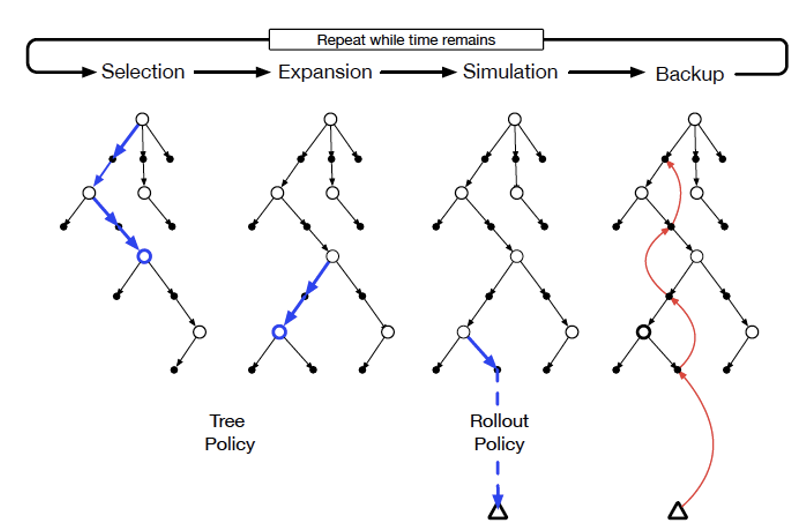
Figure B1: Illustration of the MCTS Algorithm
MCTS is a technique for building Decision Trees while starting from an initial state. The algorithm also specifies the best path through the tree. MCTS proceeds in four steps, as shown in Fig. B1, which are as follows:
- Selection: Assume that the MCTS tree has already been built up to the extent shown in the LHS figure. As usual the white circles correspond to states while the black dots represent actions (at the start of the tree building, only the Root State at the top exists). The tree consists of two kinds of states: (1) States in which all possible actions have been explored, for example the Root State and the child state to the left after the Root State, (2) States in which some or all of the actions still need to be explored. The Agent plots a course through this partially built tree, until it comes to a state in which not all actions have been evaluated, as shown the blue arrows. At each of these states, an action is chosen based on the following criteria:
- Expansion: The Selection step ends when the agent comes to a state with partially explored actions. At this point, the agent expands the tree by adding (one or more) states to the tree, as shown in the figure. The new state in turn will have one or more unexplored actions of its own. The agent chooses ones of these states and then goes to the Simulation step.
- Simulation: This step of the MCTS algorithm consists of building out the rest of the tree starting from the state that was chosen in the Expansion step. The build consists of taking successive actions, until the system enters a Terminal State. The actions are chosen using a Rollout Policy, which is usually a simple rule such as chose an action at random (since none of these Actions have been evaluated yet).
- Back-Propagation: The Backpropagation step consists of updating the $Q(S,A)$ values of all the State-Action pairs that were encountered in the path from the Root State all the way down to the Terminal State. These updates proceed backwards, starting from the Terminal State, using the following update equation:
Typically the MCTS tree building continues until a pre-determined number of iterations is reached. Once this threshold is reached, the final trace through the tree is constructed. This can be done using one of several methods, such as:
- Choose the action with the highest Q value
- Choose the path that yields the highest reward, or
- Choose the leaf node that has been visited the most
There is a variation of the MCTS algorithm, that was proposed in the AlphaZero paper by Deep Mind, that does not go through the Simulation step. Instead the leaf state is assigned a value using a Neural Network that has been trained for this purpose.