Convolutional Neural Networks
Introduction
Test Convolutional Neural Networks or ConvNets were originally invented to do image processing. Their origin lies in the research done by Hubel and Wiesel in the 1960s on the visual perception systems in cats, which later won them a Nobel Prize (see 1959; 1962; 1968). Fukushima was inspired by their work and created a neural network model which he called the NeoCognitron, see Fukushima (1975); Fukushima (1980). This model was very similar model to modern ConvNets in its structure, however it lacked an efficient training algorithm, such as Backprop. LeCun, Bottou, Bengio, Haffner (1998) later put the two pieces of the puzzle together while working at Bell Labs during the 90s, and created the modern ConvNet, whose design was based on the NeoCognitron, and which could also be trained using Backprop. LeCun’s system, called LeNet5, was successfully commercially deployed to read handwritten signatures in checks. Research in ConvNets lay dormant until 2012, when they were used for the winning entry in the ImageNet Large Scale Visual Recognition Competition (ILSVRC), see ILSVRC (2015). This also coincided with a resurgence of interest in neural networks, and since then ConvNets have led the field as the technology behind some of the most powerful DLNs.
Why Dense Feed Forward Networks don’t work well for Images
We start by first considering the question: Why do Dense Feed Forward Networks, not work well when the input is an image? There are two main reasons:
-
Consider a typical image consisting of $200 \times 200 \times 3$ pixels, which corresponds to 3 layers of $200 \times 200$ numbers, one for each of the colors Red, Green and Blue. Since the input consists of $120,000$ numbers, these many weights are needed for each node in the first Hidden Layer of a Dense Feed Forward Network. Given a typical Dense Network with say $100$ nodes in the first layer, this corresponds to 12 million weight parameters needed to describe just this layer. More parameters mean that more training data is required to prevent overfitting, which also leads to more time needed to train the model. On the other hand, when ConvNets are used to process images, it reduces the number of parameters by more than two orders of magnitude, thus improving accuracy and reducing training times. It has also been observed in practice that the accuracy of Dense Feed Forward Networks does not keep improving as more hidden layers are added, usually max-ing out at 4 to 5 layers. ConvNets however improve their accuracy with more hidden layers, indeed the most advanced ConvNet architecture features 150 layers!
-
Processing by Dense Feed Forward Networks requires that the image data be transformed into a linear 1D vector. This results in a loss of structural information, such as correlation between pixel values that are in proximity of each other in 3D. ConvNets on the other hand are able to process the original 3D image data, which makes it easier for them to recognize shapes using template matching.
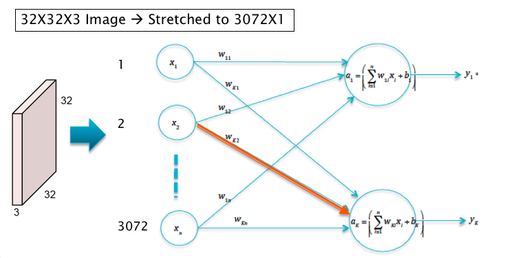
Figure 1
In order to motivate the design of ConvNets, consider the case when the input consists of $32\times 32\times 3$ CIFAR-10 images, which have to be classified into one of ten categories. Also assume that these images are processed by a Linear Neural Network Model of the type shown in Figure 1. The logits $a_k, i\le k\le 10$ in this model are given by
\[a_k = \sum_{i=1}^{3072} w_{ki} x_i + b_k,\ \ 1\le k\le 10\]Note that the sum \(\sum_{i=1}^{3072} w_{ki} x_i\) is maximized if $w_{ki} = x_i,\ 1\le i\le 3072$ under the contraint that both of these are unit vectors. Hence this lends itself to the interpretation that for each category $k$, the weights $w_{ki}, 1\le i\le 3072$ are a template or filter for the category $k$ object, which looks for images that resemble the filter itself. Hence the classification operation can be interpreted as template matching with the input image, as shown in Figure 2.
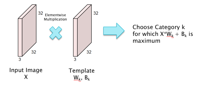
Figure 2
This template matching interpretation of Linear Filtering naturally leads to the following idea for improving the system: Instead of using a template that tries to match the entire image, why not use smaller templates that try to match objects in smaller local portions of the image. This has the following benefits: (a) Smaller templates need a smaller filter size and thus fewer parameters, and (b) Even if the object being detected moves around the image, the same template or filter can still be used, thus leading to translational invariance. This is the main idea behind ConvNets as illustrated in Figure 3.
Architecture of ConvNets
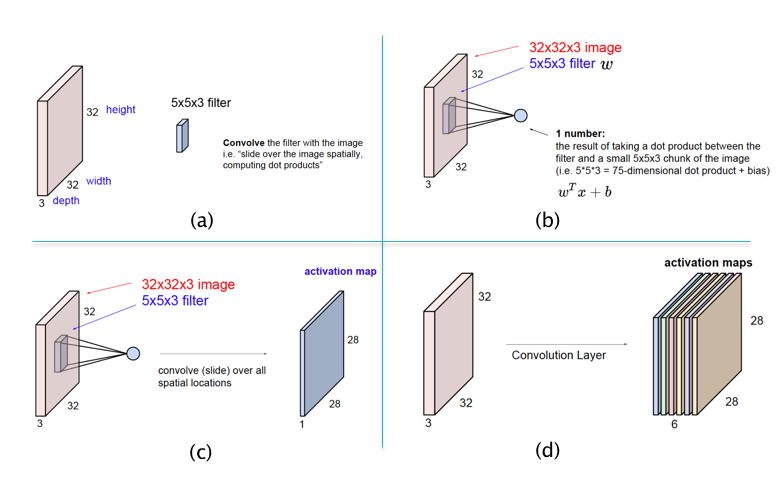
Figure 3
The main architectural aspects of ConvNets are illustrated in parts (a) - (d) of Figure 3:
-
Part (a) of Figure 3 illustrates the difference between template matching in ConvNets vs Dense Feed Forward Networks as shown in Figure 2: ConvNets use a template (or filter) that is smaller than the size of the image in height and width, while the depths match. In the example shown in (a), a filter of size $5\times 5\times 3$ is used for an image of size $32\times 32\times 3$.
-
Part (b) shows the template matching operation in ConvNets. As shown here, the matching is done locally, for possibly overlapping patches of the image. At each position of the filter, the template matching is done using the following equation to compute the pre-activation $a$ and activation $z$:
-
In this equation the pixel values $(x_1,…,x_{75})$, known as the Local Receptive Field, correspond to the local image patch of size $5\times 5\times 3$ and changes as the filter is moved around (while the filter values $w_i$ and $b$ remain unchanged). Note that the filter now only has $5\times 5\times 3 + 1 = 76$ parameters, as opposed to the $32\times 32\times 3 + 1 = 3073$ parameters that were needed for the filter in Figure 2. Both the filter as well as the local image patch are 3-D tensors, though the multiplication in Equation (1) uses a stretched out vectorized versions of the two tensors.
-
Part (c) of the figure shows the filter being moved across the image, and at each position Equation (1) is used to compute a new value of $z$, and this generates a matrix of size $28\times 28$. This matrix is known as an Activation Map (also called a Feature Map). This operation of sliding the filter across the image, while computing the dot product (1) at each position, is called a convolution. Using the same Filter for all the nodes in the Activation Map implies that all nodes in the Map are tuned to detect the same feature in the Input Layer, only at different positions in the image. This leads to the conclusion that ConvNets possess the property of Translational Invariance, i.e., they are able to detect objects irrespective of their location in the image.
-
Note that so far we have used a single filter which is only capable of detecting a single pattern in the input image. If we wish to detect multiple patterns, then we need multiple filters, each of which results in its own Activation Map, as shown in Part (d) of Figure 3. For example, Activation Map 1 may detect horizonal edges while Activation Map 2 detects vertical edges etc. As shown, a Hidden Layer in ConvNets consists of a stack of Activation Maps.
The filter in Dense Feed Forward Networks spans the entire input image, which means that it is looking for patterns that also span the entire image. However, real world images are built from smaller patterns that rarely span the entire image plane. Hence, by reducing the size of the filter, Convnets are better positioned to detect smaller shapes, which are then composed hierarchically into larger shapes and objects as we go deeper into the network. Also the Translational Invariance property ensures that the shape is detected irrespective of its location in the image plane.
Fully Connected DLNs vs ConvNets
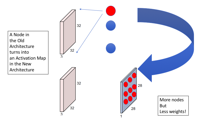
Figure 4
Figure 4 illustrates another way to contrast ConvNets with Dense Feed Forward networks. The top part of the figure shows a Dense Feed Forward Network with the input image and the nodes in the first Hidden Layer. A node in this Hidden Layer is activated if it detects a particular pattern in the image, with each node looking for a different pattern. As shown in the bottom half of the figure, with ConvNets, each of the Hidden Layer nodes is replaced by an Activation Map with multiple “sub-nodes”. The activation value at each sub-node in an Activation Map is computed using a local filter which looks for the same pattern in different parts of the image. Hence in general we need as many Activation Maps in a ConvNet as there are nodes in a Hidden Layer of a Dense Feed Forward Network. This figure also illustrates that ConvNets reduce the number of weights in the model at the expense of increasing the number of nodes. The increase in nodes causes the cost of computation to go up, but this is a worthwhile tradeoff to make since the reduction in the parameters makes the model easier to train with a smaller number of training examples.
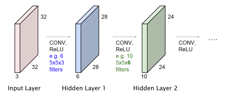
Figure 5
So far we have only described the operation of the Input Layer and the first Hidden Layer of the ConvNet. However it is straightforward to extend this design to multiple Hidden Layers, as shown in Figure 5. Just as in Fully Connected Deep Feed Forward Networks, Activation Maps in the initial hidden layers detect simple shapes, which are then built upon in an hierarchical way by the later layers to detect more complex shapes. The following hyper-parameters have to be chosen with each additional layer:
- The number of Activation Maps to be used in the Hidden Layer
- The size of the Filter and the Stride size (defined below), to be used to compute the Activations.
In the example in Figure 5, we added a second Hidden Layer with 10 Activation Maps, that are generated using a filter of size $5\times 5\times 6$. Note that the depth of this filter is not a free variable since it has to equal to the number of Activation Maps in the previous layer.
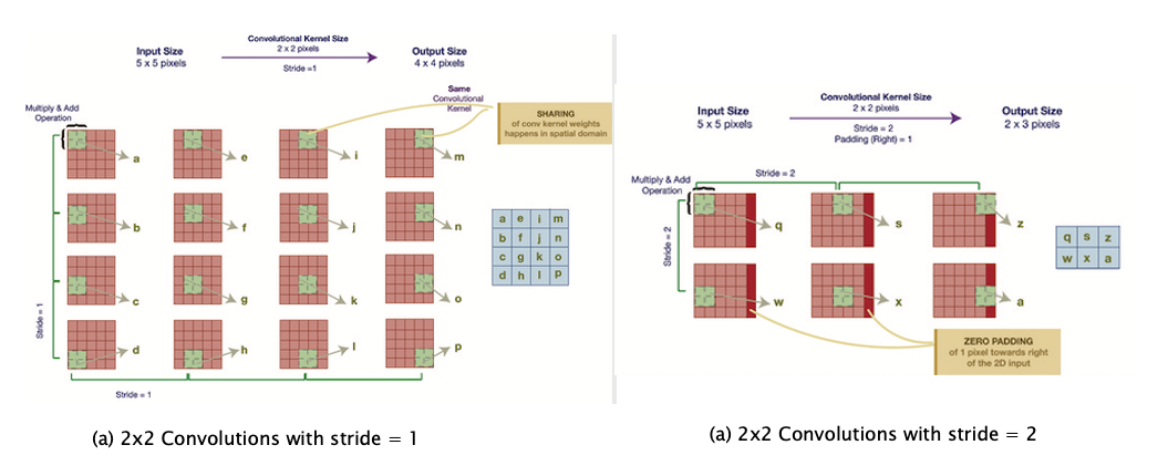
Figure 6
The computations carried out to generate an Activation Map are shown in greater detail in Parts (a) and (b) of Figure 6. Part (a) shows a Filter of size $2\times 2$, operating on an input of size $5\times 5$ (without the depth dimension). In order to generate the activations, the filter is moved by one pixel at a time, horizontally and vertically, which results in an Activation Map of size $4\times 4$. As we slide the $2\times 2$ patch across the Input Layer, we compute a dot product of the activations in the Local Receptive Field with the filter weights. An important parameter used in this process is called the Stride, denoted by $S$, and is defined as the number of pixels by which the filter is moved after each computation, either horizontally or vertically. Note that the example in Part (a) corresponds to $S = 1$ while Part(b) shows the case $S = 2$. Note that for the case $S=2$, the last column in the input feature map is not accessed (shown in red). In order to remedy this, we add a an extra column of zeroes to the right, which results in an output of size $2\times 3$. This is known as Zero Padding and is discussed further later in this chapter.
Assuming that the $r^{th}$ Hidden Layer is processed using a filter of size $L\times W\times D$, note that this filter requires $L \times W \times D + 1$ parameters. However, since the same filter is used for all the nodes in the Layer $r+1$ Activation Map, it results in a huge reduction in the number of parameters needed to describe ConvNets. Since each Activation Map in Layer $r+1$ requires its own filter, so that if there are $C$ such Maps (i.e., Layer $r+1$ is of depth $C$), then the total number of parameters needed is given by $C \times (L \times W \times D + 1)$.
In order to appreciate the scale of the reduction in number of parameters due to shared filters, consider a ConvNet with Input Layer consisting of $32\times 32\times 3$ images and containing a Hidden Layer with 20 Activation Maps generated using $5 \times 5$ filters. Since each Activation Map requires $5 \times 5\times 3+1=76$ filter parameters, $76 \times 20 = 1520$ parameters are sufficient to generate the Hidden Layer. On the other hand, in a Fully Connected Deep Feed Forward architecture with $32\times 32\times 3 = 3072$ nodes in the Input Layer and 20 nodes in the Hidden Layer, a total of $3072\times 20+20 = 61,460$ parameters are needed.
Pooling
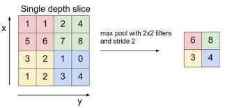
Figure 7
In addition to the Convolution operation described above, ConvNets also feature an operation called Pooling (see Figure 7). Pooling usually occurs after a Convolutional Layer, and can be described as condensing the information from that layer into a smaller number of activations. As shown in the figure, Pooling involves replacing a set of activations within a region of the Activation Map (which is just like a Local Receptive Field), by a single number. Usually the maximum of the activation values in the Local Receptive Field is used for pooling (called max-pooling), but other functions can also be used, such as the $L_1$ or $L_2$ norm. Unlike in Local Receptive Fields used in Convolutions, the corresponding fields used for the Pooling operation do not overlap. Note that the addition of Pooling does not introduce any new parameters to the ConvNet and the total number of parameters in the model are reduced considerably due to this operation.
In order to understand the Pooling operation, note that the numbers in an Activation Map that results from the Convolution operation, correspond to the likelihood of whether a particular shape or pattern is present in various locations in the previous layer. By doing Pooling right after Convolution, we throw away some of that information, which is the same as saying that the network does not care about the exact location of a pattern, it only needs to know whether the pattern is present or not. It should also be mentioned that as more processing power becomes available, some modern ConvNets, such as ResNet and the Google Inception Network, no longer incorporate Pooling in their design.
Global Max Pooling
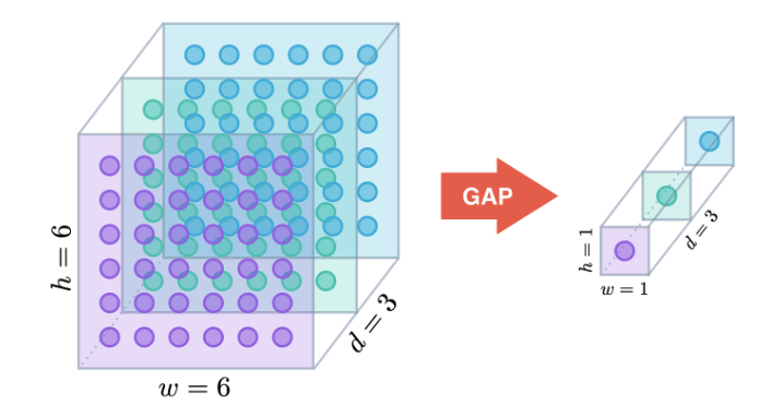
Figure 8
The output of the last convolutional layer in a ConvNet is fed into a Dense Feed Forward network before being sent into the logit layer (see Figure 9 below for an example). The traditional way of doing this is by flattening the ConvNet tensor, which causes a huge increase in the number of parameters. It is well known that more parameters can cause overfitting, unless the size of the training dataset is also increased.
In order to reduce the number of parameters, more recently models have started using the Global Max Pooling operation for this interface, which is illustrated in Figure 8. As shown, each spatial layer of the ConvNet is converted into a single node in the Dense Feed Forward network by using the max operation (or alternatively the average operation).
This design can be justified as follows: Each plane in the final ConvNet layer contains information about the presence of a pattern, and the nodes within the layer contain information the spatial location of the pattern. Since we are not interested in the spatial part of this information when doing classification, it makes sense to summarize the presence/absence information by using the maximum value of the nodes within the plane.
A Complete ConvNet
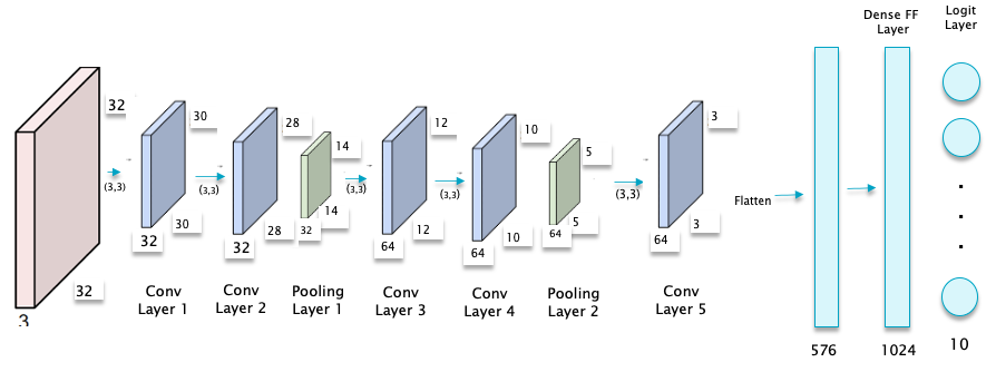
Figure 9
Figure 9 puts all the elements of a ConvNet together to come up with a network for the case when the input consists of $32\times 32\times 3$ pixel CIFAR-10 images. This network consist of the following:
- Five convolutional layers
- Two Max Pooling Layers, which occur after the second and fourth convolutional layers respectively.
- One Dense Feed Forward Layer, consisting of 1024 nodes, that is placed after the convolutional layers. Note that the output of the fifth convolutional layer is flattened, i.e., it is re-shaped from a 3D tensor of shape (3,3,64) to a 1D tensor of shape 576.
- An Output Logit Layer with 10 nodes, corresponding to the 10 categories that the input image can belong to.
- The Filters are all of spatial size (3x3).
At a high level, the convolution operation changes the representation of an image, starting from raw pixels at one end, to higher level representations using successive layers of filtering. In abstract space, as the system goes through multiple Convolutional Layers, it is basically performing non-linear transformations so that images with similar objects are clustered closer to each other in the higher level transform space. This enables the classification operation to happen using a simple linear classifier in the final layer of the network. The Fully Connected layer that is just prior to the Output Layer contains a 1024-dimensional representation of the input image. It is often used in other Deep Learning architectures that need a high level image representations.
The following code module in Keras has an implementation of the network from Figure 9.
model = models.Sequential()
model.add(layers.Conv2D(32, (3, 3), activation='relu', input_shape=(32, 32, 3)))
model.add(layers.Conv2D(32, (3, 3), activation='relu'))
model.add(layers.MaxPooling2D((2, 2)))
model.add(layers.Conv2D(64, (3, 3), activation='relu'))
model.add(layers.Conv2D(64, (3, 3), activation='relu'))
model.add(layers.MaxPooling2D((2, 2)))
model.add(layers.Conv2D(64, (3, 3), activation='relu'))

model.add(layers.Flatten())
model.add(layers.Dense(1024, activation='relu'))
model.add(layers.Dense(10, activation='softmax'))
The first convolutional layer is invoked using Conv2D(32,(3,3),activation=’relu’, input_shape=(32,32,3)). Hence it accepts as input a 3D tensor of shape (32,32,3) and filters the input using 32 filters, each of which is of shape (3,3,3). Note that only the spatial dimensions (3,3) of the filters need be specified, since the depth dimension is automatically set to the depth of the incoming tensor. This layer transforms the input tensor shape (32,32,3) into an output tensor of shape (30,30,32), and these are also the dimensions of this layer. In the next section we will show how to compute the dimensions of the tensor output from a convolutional layer, given an input tensor. As expected the 2x2 MaxPooling layer halves the spatial dimensions of the incoming tensor, but leaves its depth unchanged. Note that there is no need to re-shape the 3D CIFAR-10 images into 1D vectors, since the convolutional network is able to process the 3D tensors in their native format.
Model: "sequential"
_________________________________________________________________
Layer (type)                 Output Shape              Param #
=================================================================
conv2d (Conv2D)              (None, 30, 30, 32)        896
_________________________________________________________________
conv2d_1 (Conv2D)            (None, 28, 28, 32)        9248
_________________________________________________________________
max_pooling2d (MaxPooling2D) (None, 14, 14, 32)        0
_________________________________________________________________
conv2d_2 (Conv2D)            (None, 12, 12, 64)        18496
_________________________________________________________________
conv2d_3 (Conv2D)            (None, 10, 10, 64)        36928
_________________________________________________________________
max_pooling2d_1 (MaxPooling2 (None, 5, 5, 64)          0
_________________________________________________________________
conv2d_4 (Conv2D)            (None, 3, 3, 64)          36928
_________________________________________________________________
flatten (Flatten)            (None, 576)               0
_________________________________________________________________
dense (Dense)                (None, 1024)              590848
_________________________________________________________________
dense_1 (Dense)              (None, 10)                10250
=================================================================
Total params: 703,594
Trainable params: 703,594
Non-trainable params: 0
_________________________________________________________________
The model.summary() command shows that the model has 703,594 parameters, of which 590,848 or 84%, occur at the Dense Feed Forward layer. Hence Flattening the last convolutional layer and feeding it to a Fully Connected layer leads to an enormous increase in the number of parameters. If we replace Flatten by the “Global Max Pooling” operation, then the parameter count goes down to 179,306 shown below. The corresponding network is illustrated in Figure 10. If the model is executed then it can be shown that there is no appreciable decrease in the performance of the model.
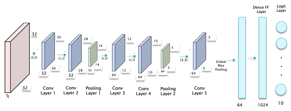
Figure 10
model = models.Sequential()
model.add(layers.Conv2D(32, (3, 3), activation='relu', input_shape=(32, 32, 3)))
model.add(layers.Conv2D(32, (3, 3), activation='relu'))
model.add(layers.MaxPooling2D((2, 2)))
model.add(layers.Conv2D(64, (3, 3), activation='relu'))
model.add(layers.Conv2D(64, (3, 3), activation='relu'))
model.add(layers.MaxPooling2D((2, 2)))
model.add(layers.Conv2D(64, (3, 3), activation='relu'))

model.add(layers.GlobalMaxPooling2D())
model.add(layers.Dense(1024, activation='relu'))
model.add(layers.Dense(10, activation='softmax'))
Model: "sequential_1"
_________________________________________________________________
Layer (type)                 Output Shape              Param #
=================================================================
conv2d_5 (Conv2D)            (None, 30, 30, 32)        896
_________________________________________________________________
conv2d_6 (Conv2D)            (None, 28, 28, 32)        9248
_________________________________________________________________
max_pooling2d_2 (MaxPooling2 (None, 14, 14, 32)        0
_________________________________________________________________
conv2d_7 (Conv2D)            (None, 12, 12, 64)        18496
_________________________________________________________________
conv2d_8 (Conv2D)            (None, 10, 10, 64)        36928
_________________________________________________________________
max_pooling2d_3 (MaxPooling2 (None, 5, 5, 64)          0
_________________________________________________________________
conv2d_9 (Conv2D)            (None, 3, 3, 64)          36928
_________________________________________________________________
global_max_pooling2d (Global (None, 64)                0
_________________________________________________________________
dense_2 (Dense)              (None, 1024)              66560
_________________________________________________________________
dense_3 (Dense)              (None, 10)                10250
=================================================================
Total params: 179,306
Trainable params: 179,306
Non-trainable params: 0
_________________________________________________________________
Sizing ConvNets
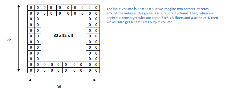
Figure 11
The size (or volume) of a Convolutional Layer in a ConvNet is related to the volume of the prior Convolutional Layer, as well as the size of the Filter used in the convolution operation, and in this section we give some simple expressions that can be used to connect the two. Before we launch into this topic, we introduce another important parameter used in ConvNet design, namely the Zero-Padding used during convolution, which we denote as $P$. Zero-Padding does the following: Instead of processing an input of size $L \times W$, we add one or more layers of zeroes around it, in both the dimensions. Hence if $P=1$ then only a single Zero-Padding layer is added, while two layers are added for the case $P=2$ (see Figure 11 for an illustration of the case $P=2$).
Sizing the Convolutional Layer
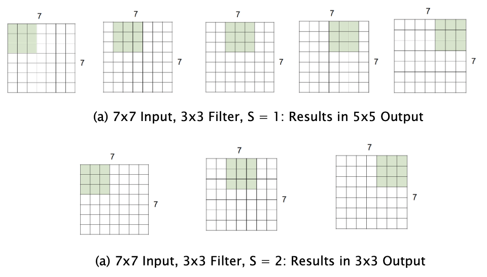
Figure 12
We will use the following notation:
- $L_r$, $W_r$, $D_r$: Length, Width and Depth dimensions of the volume in layer $r$
- $F_r$: Size of the Filter used when going from layer $r$ to $r+1$
- $P_r$: Amount of Zero Padding used for layer $r$
- $S_r$: The Stride size used in the layer $r$ to layer $r+1$ filter.
It can then be shown that
\[W_{r+1} = {W_r - F_r + 2P_r\over{S_r}} + 1\] \[L_{r+1} = {L_r - F_r + 2P_r\over{S_r}} + 1\]In order to gain insight into this formula, consider Figure 12:
- First consider the case $S_r = 1, P_r=0$: As shown in Part (a) of the figure, $W_r - F_r$ is the number of spaces by which the filter can be slid from left to right with a stride of 1. With the addition of $1$ to account for the final position of the filter, we get $W_{r+1} = W_r - F_r +1$. The presence of zero padding of size $P_r$ results in an increase of the size of the feature map by $2P_r$, so that $W_{r+1} = W_r - F_r + 2P_r + 1$
- If the stride $S_r > 0$, then the number of spaces by which the filter can be moved becomes $W_{r+1} = {W_r - F_r + 2P_r\over{S_r}} + 1$
In the presence of parameter sharing, $F_r\times F_r\times D_r + 1$ filter weights are required per Activation Map in layer $r+1$, for a total of $D_{r+1}\times (F_r \times F_r \times D_r +1)$ weights and $D_{r+1}$ biases.
As an example of the application of this formula, consider the following example: $W_r=10, F_r= 3, S_r=2$ with no zero padding, so that $P_r=0$. Then applying the above formula it follows that $W_{r+1} = 4.5$, which being a non-integer implies that it is not possible to fit an integer number of nodes in layer $r+1$. We can change the stride to $S_r=1$ which leads to $W_{r+1}=5$, thus resulting in a valid architecture.
In modern ConvNet design, zero padding is used most often to ensure that the volume sizes remain unchanged as we move deeper into the network, in other words we would like that $W_{r+1}=W_r, L_{r+1}=L_r, D_{r+1}=D_r$. From the above equation, this can be ensured if the stride $S_r=1$ and the zero padding $P_r$ is chosen to be:
\[P_r = {F_r - 1\over 2}\]The most common ConvNet filter sizes are $F_r = 3$ and $F_r = 5$, which results in $P_r = 1$ and $P_r = 2$ respectively. As we will see later in this chapter, some of the advanced ConvNet designs such as VGGNet and ResNet keep the size of the volumes fixed in their Convolutional Layers, which helps in producing networks with hundreds of layers. In the absence of this feature, the volume sizes progressively decrease as we move deeper in the network, thus limiting the number of Hidden Layers to much smaller values. Zero Padding is implemented in Keras using the command: conv = model.add.layers.Conv2D(6, (3,3), strides=2, padding=’same’).
As we will see later, early ConvNet designs featured bigger Filters, such as $11\times 11$ or $7\times 7$, in their first few layers. However in more recent designs, it has been discovered that using smaller $3\times 3$ filters, even in the first layer, leads to better performance, as well as a reduction in the number of parameters. This aspect of ConvNet design is explored more fully in Section SmallFilters. The depth $D_r$ is usually chosen to be a power of $2$ for computational reasons: Numerical routines used in the calculations work more efficiently in this case.
Sizing the Pooling Layer
If Layer $r+1$ is a Pooling Layer, then the following formulae hold (using the same notation as in the prior section):
\[W_{r+1} = \frac{W_r-F_r}{S_r} + 1\] \[H_{r+1} = \frac{H_r-F_r}{S_r} + 1\] \[D_{r+1} = D_r\]Note the following:
-
The Pooling Layer does not lead to the introduction of new parameters.
-
It is not common to use Zero Padding as part of Pooling, hence the absence of the $P_r$ term in the above equations.
-
Common numbers used for Pooling are $F_r = 2, S_r = 2$ or $F_r = 3, S_r = 2$.
Computations during Convolutions
Using the same notation as above, the number of multiplications needed to generate all the activations in Layer $r+1$ is given by:
\[Mult = F_r F_r D_r\times W_{r+1} H_{r+1}\times D_{r+1}\]This can be understood as the product of the following factors:
- The number of computations required to generate a single element of an Activation Map in layer $r+1$ = $F_r F_r D_r$
- The number of computations required to generate all the elements of a single Activation Map = $F_r F_r D_r \times W_{r+1} H_{r+1}$
- The number of computations required to generate all the $D_{r+1}$ Activation Maps in layer $r+1$ = $F_r F_r D_r \times W_{r+1} H_{r+1} \times D_{r+1}$
Earlier in this chapter we observed that a ConvNet Layer with $D$ Activation Maps is roughly equivalent to a Dense Feed Forward Network Layer with $D$ nodes. Given two Dense Feed Forward Layers with $D_r$ and $D_{r+1}$ nodes respectively, the number of computations required to generate the $D_{r+1}$ activations in layer $r+1$ is given by $D_r D_{r+1}$. It follows that the number of computations required to generate Layer $r+1$ in a ConvNet is greater than the corresponding number in a Dense Feed Forward Network by a multiplicative factor equal to $F_r F_r \times W_{r+1} H_{r+1}$, i.e., the size of the ConvNet Filter times the size of the Activation Map. This accounts for the large increase in computation time that we observed in the ConvNet model earlier in the chapter.
One Dimensional ConvNets
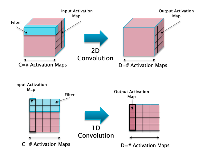
Figure 13(a)
2D Convolutional Networks are ideal to do Image Processing, since they are able to process 3D image tensors in their native format. But there are important datasets that are either 1D or 2D tensors, examples include:
- Natural Language Processing: Sentences can be represented as a 2D tensor, with a row for each word and the columns with the feature representations for the corresponding word.
- Structured Tabular Datasets: These are the most common type of datasets, and can be either a 1D vector or a 2D matrix.
The idea of doing local filtering using convolutions can be extended to these types of datasets by used 1D Convolutions, as shown in Figure 13(a). The bottom part of the figure shows a 1D Convolution using a 2x1 filter with a depth of 4 (in blue). An Activation Map in this case is no longer a 2D matrix, but instead is a 1D vector. The 1D Convolutions acts on the 1D Input Activation Map, and converts into an output 1D Activation Map, as shown. If there are 4 such 1D filters, then each of them will generate its own output Activation Map, resulting an output of tensor shape (4,4) as shown.
The process of sliding (or convolving) the 2x1 filter across the input is illustrated in Figure 13(b). It is easy to see that the formula $ W_{r+1} = \frac{W_r-F_r+2P_r}{S_r}+1 $ that was derived for the size of the output Activation Map in 2D Convolutions continues to hold for this case as well.
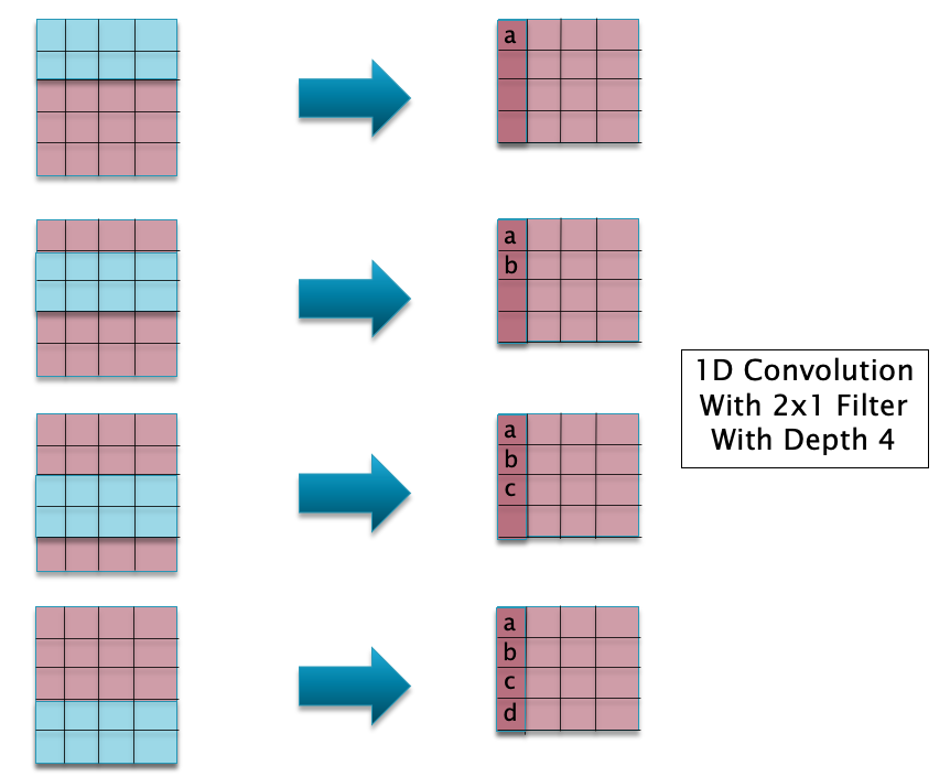
Figure 13(b)
The 1D Convolutional model to process the IMDB Moview Review dataset is illustrated in Figure 14. The Embedding Layer converts each review from a 1D vector of integers of size 500, into a 2D matrix of shape (500,128), with rows representing words from the review in vector format. The 128 size embedded vector representation for the words is learnt as part of the training.
Note that a Flatten Layer is no longer needed unlike for the case of Dense Feed Forward Networks, since the 1D ConvNet model is capable of processing the text input in its native 2D format.
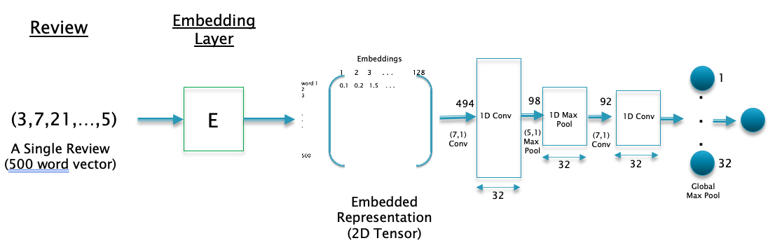
Figure 14
The Keras code for this model is given next.
model = Sequential()
model.add(layers.Embedding(max_features, 128, input_length=max_len))
model.add(layers.Conv1D(32, 7, activation='relu'))
model.add(layers.MaxPooling1D(5))
model.add(layers.Conv1D(32, 7, activation='relu'))
model.add(layers.GlobalMaxPooling1D())
model.add(layers.Dense(1))
model.summary()
Model: "sequential_4"
_________________________________________________________________
Layer (type)                 Output Shape              Param #
=================================================================
embedding_2 (Embedding)      (None, 500, 128)          1280000
_________________________________________________________________
conv1d_4 (Conv1D)            (None, 494, 32)           28704
_________________________________________________________________
max_pooling1d_2 (MaxPooling1 (None, 98, 32)            0
_________________________________________________________________
conv1d_5 (Conv1D)            (None, 92, 32)            7200
_________________________________________________________________
global_max_pooling1d_2 (Glob (None, 32)                0
_________________________________________________________________
dense_6 (Dense)              (None, 1)                 33
=================================================================
Total params: 1,315,937
Trainable params: 1,315,937
Non-trainable params: 0
_________________________________________________________________
Transfer Learning with ConvNets
When ConvNets are trained on image data, such as ImageNet, we have the luxury of having a database of millions of labeled images, which enables us to train fairly large networks with hundreds of layers to a high degree of accuracy. These networks, examples of which include ResNet, VGGNet, or Google InceptionNet, take multiple weeks to train, and involve huge amounts of advanced computing resources such as GPUs, to do so (the architecture of these networks is discussed later in this blog).
Practitioners often run into problems when there are not enough training examples to train such large networks, or if they don’t have access to the necessary computing resources for the particular problem that they are trying to solve. Fortunately there is a technique called Transfer Learning that enables us to develop accurate models even without a lot of training data or computing resources. Transfer Learning enables us to transfer the parameters learnt from training a model for Problem 1, to be re-used in the model for another Problem 2, provided the training dataset for Problem 2 is similar to that used for Problem 1.
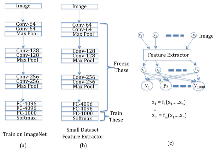
Figure 15
In order to understand how Transfer Learning works, consider Figure 15. Part (a) of the figure shows a traditional ConvNet, say ConvNet 1, which has been trained on a large dataset such as ImageNet. It has a mixture of Convolutional and Maxpool layers, which is followed by Dense Feed Forward layers at the end of the network. In order to reuse the parameters learnt from this network, to another network, say Convnet 2, with a similar dataset which is much smaller in size, we do the following:
-
As shown in Part (b) of Figure 15, we freeze the parameters of ALL the layers of ConvNet 1, except for the Logit Layer (called FC-1000), and then use these parameters as a Feature Extractor in ConvNet 2. Note that ConvNet 2 (shown in Part(c)) corresponds to a simple Logistic Regression model with a Feature Extractor used in the Input Layer.
-
In order to complete ConvNet 2, we only need to find the weights of the connections between the Feature Extractor outputs ${z_i}$ and the Output Layer ${y_i}$, as shown in Part (c) of Figure 15. Since the number of trainable weights are now much smaller, they can be estimated using the smaller dataset available for ConvNet 2 with smaller compute resources.
The Transfer Learning technique described above has been shown to be very effective in solving Image Processing problems, and has enabled the use of sophisticated ConvNet Models for a wider modeling community.
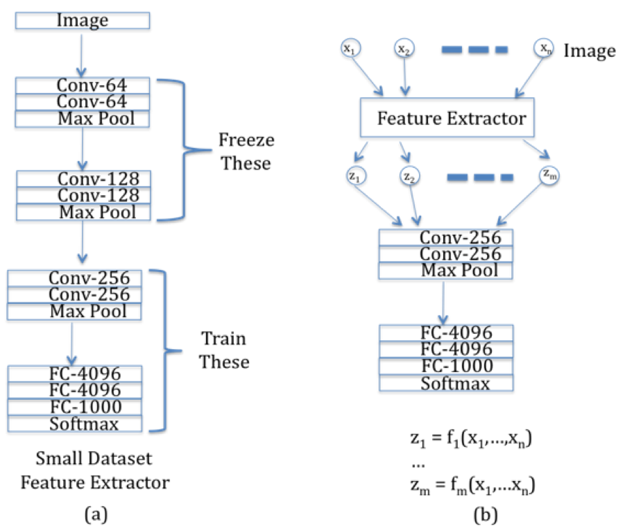
Figure 16
If larger datasets are available for Problem 2 (but which are still smaller than ImageNet in size), then the technique that was explained above, can be extended to networks with additional layers, as shown in Figure 16). In this case we reduce the number of frozen layers from ConvNet 1, so that ConvNet 2 now has additional layers that need to be trained. Once again the frozen layers in ConvNet 1 act as a Feature Extractor whose outputs are fed into the rest of the convolutional network.
Why does Transfer Learning work so well? A ConvNet trained on a large dataset such as ImageNet, learns to recognize generic patterns and shapes that also occur in non-ImageNet data. In addition, even non-image data, such as audiowave signals, can be classified well with the patterns that are learnt with ImageNet. A general rule of thumb is that the earlier Hidden Layers in the ConvNet contain the more generic portion that can be re-used in other contexts, and the model becomes more and more specific to the particular dataset, as we go deeper into the network. In practice, researchers can save a large amount of time (and money), by not starting from scratch, but instead use an appropriate pre-trained model, when they start working on a new model.
There are two ways in which features from image datasets can be extracted:
- All the images in the dataset (training, validation and test) are fed into base model, and the final tensors are used as the new image representation. Note that the original images are no longer used in the rest of the model training and validation.
- The model incorporates both the pre-trained base model as well as the trainable portion. Training is done using the image dataset, during which the weghts in the pre-trained portion are frozen.
Method 1 leads to faster training, since the images don’t have to be processed by the large MobileNet model. However it precludes the use of data augmentation. Method 2 on the other hand is slower since each image passes through the conv-base in the forward pass, however it allows the user to create new images on the fly during training using data augmentation.
In the following example we will use Method 1.
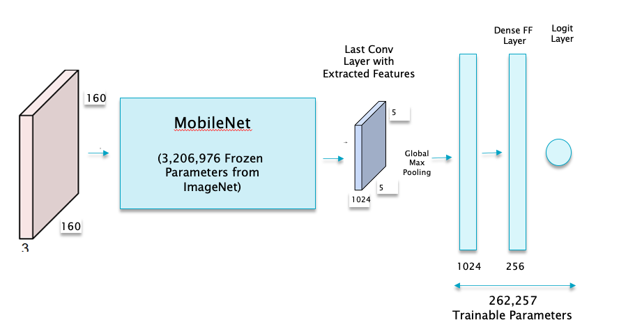
Figure 17
The complete model is shown in Figure 17. During the pre-training phase, each image is passed through the MobileNet model, and its final output of shape $5\times 5\times 1024$ is stored as the new training dataset. These extracted features are then converted into a vector using the Global Max Pooling operation and then sent through a simple Dense Feed Forward model with a single hidden layer with 256 nodes.
Model: "model_2"
_________________________________________________________________
Layer (type)                 Output Shape              Param #
=================================================================
input_5 (InputLayer)         [(None, 5, 5, 1024)]      0
_________________________________________________________________
flatten_3 (Flatten)          (None, 25600)             0
_________________________________________________________________
dense_11 (Dense)             (None, 256)               6553856
_________________________________________________________________
dropout_2 (Dropout)          (None, 256)               0
_________________________________________________________________
dense_12 (Dense)             (None, 1)                 257
=================================================================
Total params: 6,554,113
Trainable params: 6,554,113
Non-trainable params: 0
_________________________________________________________________
The Transfer Learning model results in validation accuracy of about 97%, which is a big improvement on the 60% accuracy in the Dense Feed Forward model without feature extraction.
Trends in ConvNet Design
The performance of ConvNets has improved in recent years due to several architectural changes, which include the following:
- Residual Connections
- Use of Small Filters
- Bottlenecking Layers
- Grouped Convolutions (also called Split-Transform-Merge)
- Depthwise Separable Convolutions
- Dispensing with the Pooling Layer
- Dispensing with Fully Connected Layers
Residual Connections are arguably the most important architectural enhancement made to ConvNets since their inception, and are covered in some detail when we discuss ResNets. Even though proposed in the context of ConvNets, they are a critical part of other Neural Network architectures, in particular Transformers.
Residual Connections
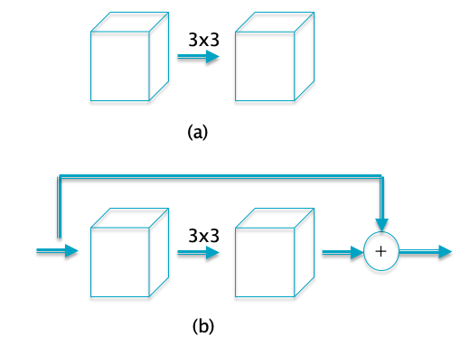
Figure 18
Residual connections are illustrated in Part (b) of Figure 18. They were introduced as part of the ResNet model in 2015 and were shown to lead to large improvement in model performance by making possible trainable models with hundreds of layers. Prior to the discovery of Residual Connections, models with more 20-30 layers ran into the Vanishing Gradient problem during training, due to the gradient dying out as it was subject to multiple matrix multiplication during Backprop.
Part (a) of the figure shows a set of regular conolutional layers, Residual Connections feature a bypass connection from the input to the output such that the input signal is added to the output signal as shown in Part(b). This design clearly helps with gradient propagation, since the addition operation has the effect of taking the gradient at the output of the sub-network and propagating it without change to the input. The idea of Residual Connections is now widely used in DLN architectures, state of the art networks such DenseNet and Transformers include it as part of their design. We provide a deeper discussion of the benefits of Residual Connections in the section on ResNets later in this chapter.
Small Filters in ConvNets
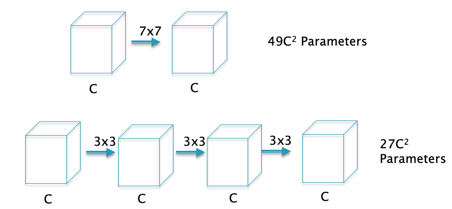
Figure 19
As ConvNet architectures have matured, one of the features that has changed over time is the filter design. Early ConvNets such as AlexNet used large $7 \times 7$ Filters in the first convolutional layer. However, a stack of $3 \times 3$ Filters is a superior design to the single $7 \times 7$ Filter for the following reasons (see Figure 19)):
-
The stacked $3 \times 3$ design uses a smaller number of parameters: Using the formula for number of parameters in a ConvNet developed in Section SizingConvnets, it follows that the $7 \times 7$ Filter uses $C \times (7 \times 7 \times C + 1)=49 C^2 + C$ parameters (since each Filter uses $7 \times 7 \times C + 1$ parameters, and there are C such Filters). In comparison the stacked $3 \times 3$ design uses a total of $3 \times C \times (3 \times 3 \times C + 1)=27 C^2 + 3C$ parameters, i.e., a 45% decrease.
-
The stacked $3 \times 3$ design incorporates more non-linearity, it has 4 ReLU Layers vs the 2 ReLU Layers in the $7 \times 7$ case, which increases the system’s modeling capacity.
-
The stacked $3 \times 3$ design results in less computation.
The better performance with smaller filters can be explained as follows: The job of a filter is to capture patterns within the Local Receptive Field and patterns at a finer level of granularity can be captured with smaller filters. Also as we stack up the layers, filters at the deeper levels progressively capture patterns within larger areas of the image. For example consider the case of the stacked $3 \times 3$ Filters in Figure 19: While the first $3 \times 3$ Filter scans patches of size $3 \times 3$ in the input image, it can be easily seen that the second $3 \times 3$ filter effectively scans patches of size $5 \times 5$, and the third $3 \times 3$ Filter scans patches of size $7 \times 7$ in the input image. Hence even though the filter size is unchanged as we move deeper into the network, they are able to capture patterns in progressively larger sections of the input image. This is illustrated in Figure 20 for the case of two layers of $3\times 3$ filters.
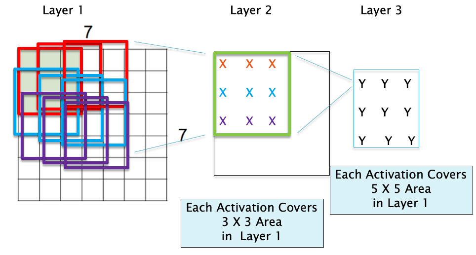
Figure 20
Bottlenecking using 1x1 Filters
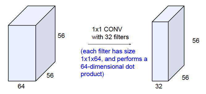
Figure 21
Several modern ConvNets use Filters of size $1\times 1$. At first glance these may not make sense, but note that because of the depth dimension, a $1\times 1$ Filter still involves a dot product with weights associated with the depth dimension and the corresponding activations across them. As shown in Figure 21, this can be used to compress the number of layers in a ConvNet. This operation called ‘bottlenecking’, is very useful and is frequently used in modern ConvNets to reduce the number of parameters or the number of operations required.
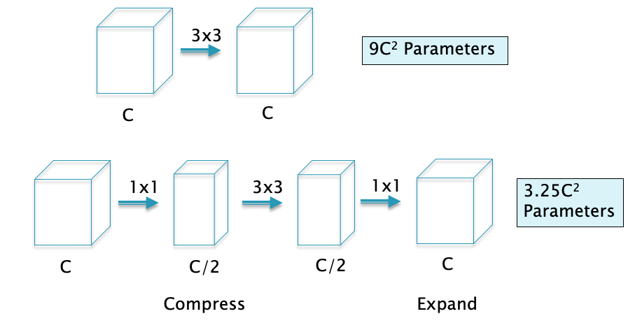
Figure 22
Bottlenecking with $1 \times 1$ and $1 \times n$ filters, as illustrated in Figure 22: As shown, the first $1 \times 1$ filter is used in conjuction with a reduction in depth to $C/2$. The $3 \times 3$ filter then acts on this reduced depth layer, which gives us the reduction in parameters, and this is followed by another $1 \times 1$ filter that expands the depth back to $C$. It can the shown that this filter architecture reduces the number of parameters from $9 C^2$ to $3.25 C^2$ (ignoring the bias parameters). It can be easily shown that the number of computations also decreases from $9C^2 HW$ to $3.25C^2 HW$, where $H,W$ are the spatial dimensions of the ConvNet.
Grouped Convolutions
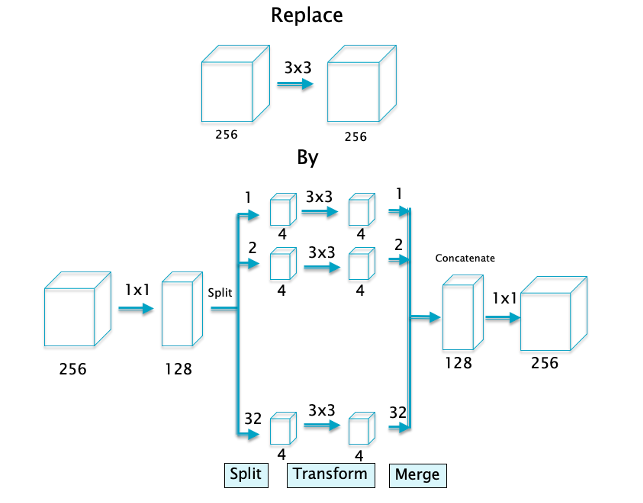
Figure 23
Grouped Convolutions are illustrated in Figure 23. As shown, the regular $3\times 3$ convolution is replaced by the following:
- Step 1: Compress the input layers using a $1\times 1$ convolution from 256 layers to 128.
- Step 2: Split the output of Step 1 into 32 separate convolution layers, such that each layer has 4 Activation Maps.
- Step 3: Use regular $3\times 3$ convolution on each of the 32 layers
- Step 4: Marge or Concatenate all 32 convolution layers to form a structure with 128 Activation Maps
- Step 5: Expand the output of step 4 to 256 Activation Maps with a $1\times 1$ convolution
Grouped Convolutions have been shown to improve the performance of ConvNets. It is not completely clear how they are able to do so, but it has been observed that the 4 Activation Maps in the smaller Convolutional Layers learn features that have a high degree of correlation. For example AlexNet, which was one of the earliest ConvNets, featured 2 groups due to memory constraints, and it was shown that Group 1 learnt black and white shapes while Group 2 learnt colored shapes. This functions as akind of regularizer and helps the network learn better features.
It can also be shown that the number of computations for the Grouped case decreases in inverse proportion to the number of groups and the size of the filter. This calculation is carried out detail in the next section.
Depthwise Separable Convolutions
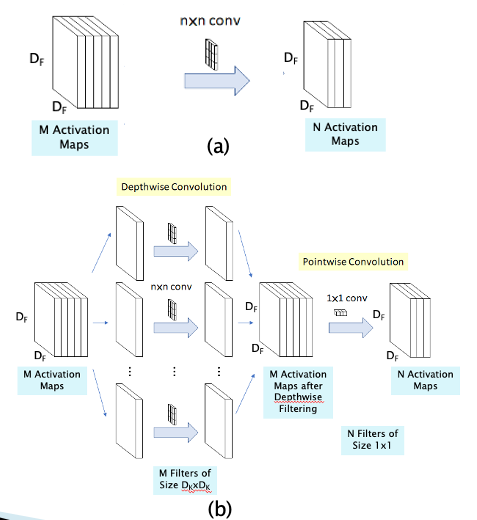
Figure 24
A standard convolution both filters and combines inputs into a new set of outputs in one step. The depthwise separable convolution splits this into two layers, a separate layer for filtering and a separate layer for combining. This factorization has the effect of drastically reducing computation and model size. Hence they take the idea behind Grouped Convolutions to the limit by splitting up the M Activation Maps in the input layer into M separate single layer Activation Maps as shown in Figure 24. Each of these Activation Maps is then processed using a separate convolutional filter, and then combined together at the output. A simple $1\times 1$ convolution, is then used to create a linear combination of the output of the depthwise layer . Hence this design serializes the spatial and depthwise filtering operations of a regular convolution. An immediate benefit of doing this is a reduction in the number of computations (and the number of parameters), as shown next:
- The number of computations in a regular convolution shown in Part (a) is given by $D_K D_K\times MN\times D_F D_F$ where $D_K$ is the size of the filter, M is the depth of the input layer, N is the depth of the output layer and $D_F$ is the size of the output Activation Map.
- The number of computations in the Depthwise Separable Convolution is given by $D_K D_K\times M\times D_F D_F + MN\times D_F D_F$
It follows that the ratio $R$ between the number of computations in the Depthwise Separable network and the Regular COnvNet is given by
\[R = {1\over N} + {1\over D_K^2}\]For a typical filter size of $D_K= 3$, it follows that the number of computations in the Depthwise Separable network reduces by a factor of 9, which can be a significant reduction for training times that sometimes run into days. The idea of separating out the filtering into two parts, spatial and depthwise, has subsequently proven to be very influential, and underlies the type of filtering in a new model called Transformers, which we will study in a later chapter.
ConvNet Architectures
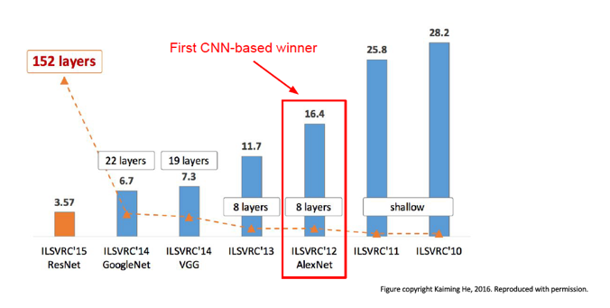
Figure 25
We briefly survey ConvNet architectures starting with the first ConvNet, LeNet5, whose details were published in 1998. Starting with AlexNet in 2012, ConvNets have won the ImageNet Large Scale Visual Recognition Challenge (ILSVRC) image classification competition run by the Artificial Vision group at Stanford University. ILSVRC is based on a subset of the ImageNet database that has more than 1+ million hand labeled images, classified into 1,000 object categories with roughly 1,000 images in each category. In all there are 1.2 million training images, 50K validation images and 150K testing images. If an image has multiple objects, then the system is allowed to output upto 5 of the most probably object categories, and as long as the the “ground-truth” is one of the 5 regardless of rank, the classification is deemed successful (this is referred to as the top-5 error rate).
Figure 25 plots the top-5 error rate and (post-2010) the number of hidden layers in Neural Network architectures for the past seven years. Prior to 2012, the winning designs were based on traditional ML techniques using SVMs and Feature Extractors. In 2012 AlexNet won the competition, while bringing down the error rate signficantly, and inaugurated the modern era of Deep Learning. Since then, error rates have come down rapidly with each passing year, and currently stand at 3.57%, which is better than human-level classification performance. At the same time, the number of Hidden Layers has increased from the 8 layers used in AlexNet, to 152 layers in ResNet which was the winner in 2015. This is when the machines outpaced humans in accuracy and the competetion was stopped.
In this section our objective is to briefly describe the architecture of the winners from the last few years, namely: AlexNet (2012), ZFNet (2013), VGGNet (2014), Google InceptionNet (2014) and ResNet (2015). The first three are “classical” ConvNet designs with multiple Convolutional, Pooling, and Dense layers arranged in a linear stack. The Google Inception Network and ResNet have diverged from some of the basic tenets of the first ConvNets, by adopting the Split/Transform/Merge and the Residual Connection designs respectively. In more recent years the focus has shifted towards coming up with ConvNets that have a much lower number of parameters, without sacrificing performance. The InceptionNet actually began this trend, and MobileNet also belongs to this category of models.
These following architectures are described in greater detail next:
- LeNet (1998)
- AlexNet (2012)
- ZFNet (2013)
- VGGNet (2014)
- InceptionNet (2014)
- ResNet (2015)
- Xception (2016)
- DenseNet (2017)
- MobileNet (2017)
The table below which is taken from Keras Documentation summarizes the size, performance, number of parameters and depth of these models. The performance is with respect to the ImageNet dataset, with the Top-1 Accuracy being the performance for the best predition and the Top-5 Accuracy being the performance for the case when the Ground Truth is among the top 5 predictions.
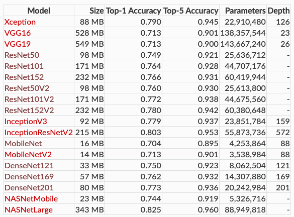
Figure 26
LeNet5 (1998)
LeNet5 was the first ConvNet, it was designed by Yann LeCun and his team at Bell Labs, see Lecun, Bottou, Bengio, Haffner (1998). It had all the elements that one finds in a modern ConvNet, including Convolutional and Pooling Layers, along with the Backprop algorithm for training (Figure 27). It only had two Convolutional layers, which was a reflection of the smaller training datsets and processing capabilities available at that time. LeCun et.al. used the system for handwritten signature detection in checks, and it was successfully deployed commercially for this purpose.
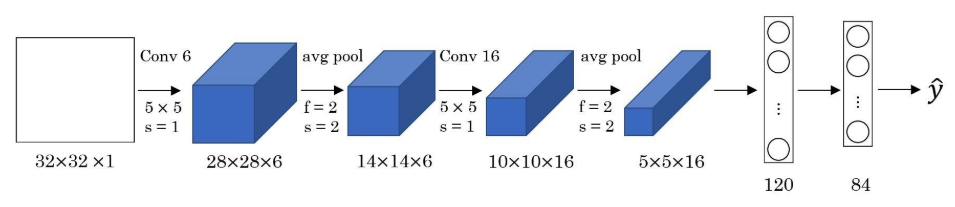
Figure 27
As shown in Figure 27, the system uses two Convolution layers with $5 \times 5$ Filters and Stride $S=1$, and two Pooling layers with $2 \times 2$ Filters and $S=2$. The system reduces the input $32 \times 32$ images into 16 Activation Maps of size $5 \times 5$ at the end of the second pooling operation, before flattening this tensor and outputting the result into the Fully Connected part of the design.
AlexNet (2012)
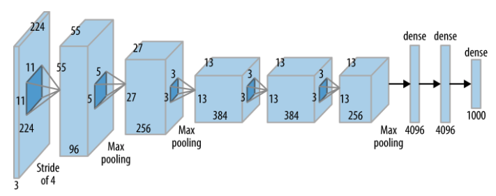
Figure 28
After the pioneering work done in LeNet5, progress in ConvNets lay dormant for more than a decade. It was held back by the following issue: In order to train larger ConvNets with millions of parameters, it was necessary to have a large training dataset with correspondingly millions of images (this is required in order to prevent overfitting). Image datasets of this size did not exist until about 2010, when the ImageNet dataset was released.
AlexNet is responsible for the explosion in interest in DLNs in the last few years.This network won the ILSVRC competition in 2012 by a wide margin compared to its nearest rival which was based on SVMs (it had a 15.4% top-5 error rate vs 26.2% for the next lowest network), and this opened up the eyes of the ML community to the potential of Deep Learning. The architecture of AlexNet Krizhevsky, Sutskever, Hinton (2012) was very similar to that of LeNet5, with the following exceptions (see Figure 28)):
-
AlexNet replaced the tanh() activation function used in LeNet5, with the ReLU function and also the MSE loss function with the Cross Entropy loss.
-
AlexNet used a much bigger training set. Whereas LeNet5 was trained on the MNIST dataset with 50,000 images and 10 categories, AlexNet used a subset of the ImageNet dataset with a training set containing 1+ million images, from 1000 categories.
-
AlexNet used Dropout regularization (= 0.5) to combat overfitting (but only in the Fully Connected Layers). It also used a Normalization Layer, that is no longer used in ConvNets since it does not improve the performance significantly.
AlexNet was able to use a training set which was larger by two orders of magnitude, without a corresponding increase in training time, by exploiting the power of GPUs. It used two GTX 580 GPUs for 5-6 days to complete the training phase. This was enabled by using a Grouped Convolution design (not shown in the above figure) with two groups, each running on its own GPU.
AlexNet used 5 Convolutional layers (vs 2 used in LeNet5), and it used a similar combination of Convolutional and Pooling Layers followed by 3 Dense Layers. The input into the system consisted of $224 \times 224 \times 3$ images, which are then processed by the first convolutional layer with 96 Activation Maps using $11 \times 11$ filters with $S=4, P=0$. The system has $4$ more Convolutional layers, consisting of a $5 \times 5$ Filter followed by three $3 \times 3$ Filters. The number of Activation Maps in the last Convolutional layer is increased to 256 before the activations are flattened and fed into the Fully Connected Layers.
AlexNet had a total of 60 million parameters, which was still much more than the number of training images available. In order to prevent overfitting, the system used Data Augmentation techniques to produce additional test images, thus boosting the Test dataset to 15 million images.
ZFNet (2013)
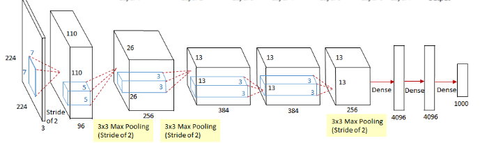
Figure 29
ZFNet, which was designed by Zeiler and Fergus (2013), won the ILSVRC competition in 2013 by achieving a 11.2% top-5 error rate. The architecture was essentially a tuning modification to AlexNet, with the following changes (Figure 29)):
-
Use of $7\times 7$ instead of $11 \times 11$ Filters in the first Convolutional layer,
-
Use of a stride of $S=2$ instead of $S=4$.
The reduction in filter size and stride helped to pick image features at a finer level of resolution.
VGGNet (2014)
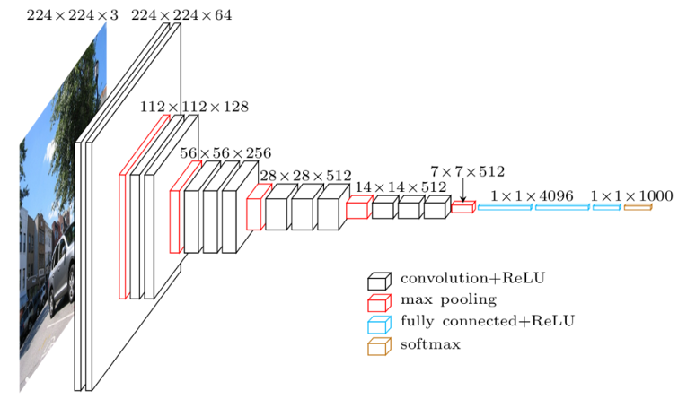
Figure 30
Simonyan and Zisserman (2014) created a network which reduced the top-5 ILSVRC error rate to 7.3% (Figure 30)). The main innovations in the network, called VGGNet, are the following:
-
VGGNet increased the number of layers to 19 layers (16 Convolutional + 3 Fully Connected), as opposed to the previous designs that were limited to 8 such layers.
-
VGGNet considerably simplified the ConvNet design, by repeating the same smaller convolution filter configuration 16 times: All the filters in VGGNet were limited to $3 \times 3$, with stride and padding of 1, along with $2 \times 2$ maxpooling filters with stride of 2. Since these smaller filters are used in a series of 2 or 3 consecutive convolutional layers, the net effect is that of using a single $5 \times 5$ or $7 \times 7$ filter, but with the advantage of a smaller number of parameters and increased model non-linearity, as explained in Section SmallFilters.
An interesting fact about about VGGNet is that it has a total of 144 million parameters, of which about 124 million parameters are used in the final 3 Dense layers. This was a result of the Flatten operation on the last 3D tensor of which when connected to the dense layer with 4096 nodes resulted in $7 \times 7 \times 512 \times 4096=102,760,448$ parameters. Global Max Pooling was used in subsequent designs to reduce this parameter count.
Even though VGGNet did not win the ILSVRC competition in 2014, it came close to doing so, and its simple and elegant design has been influential in subsequent ConvNet architectures. The main lesson from VGGNet was the classical ConvNet design of the LeNet5/AlexNet type can be substantially improved by increasing the number of Convolutional Layers and by using smaller filters.
Google Inception Network (2014)
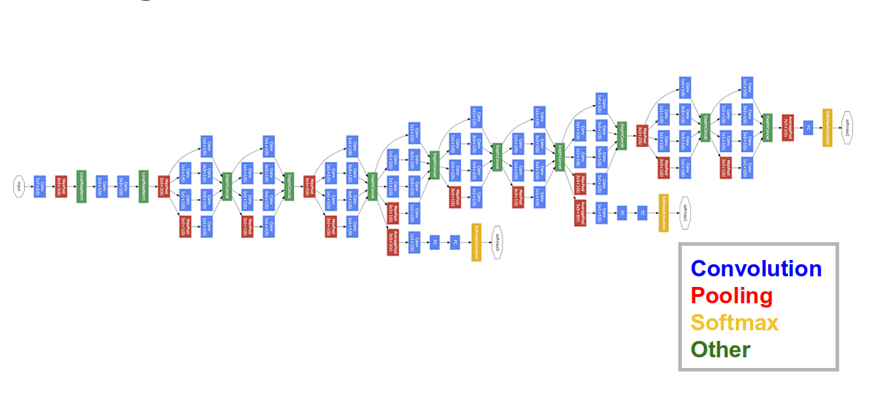
Figure 31
Along with VGGNet, the Google Inception Network (Figure 31)) competed in the 2014 ILSVRC competition, see Szegedy, Ioffe, Vanhoucke (2016). It did slightly better than VGGNet (6.7% top 5 error rate as compared to 7.3% for VGGNet), but at the cost of a more complex architecture. The Inception Network was the first design that moved away from the linear stacking of convolutional and pooling layers and introduced the Split/Transform/Merge architecture to ConvNets. It was able to reduce the number of parameters to about 5 million by using this and also by eliminating all fully connected layers with the use of Global Max Pooling.
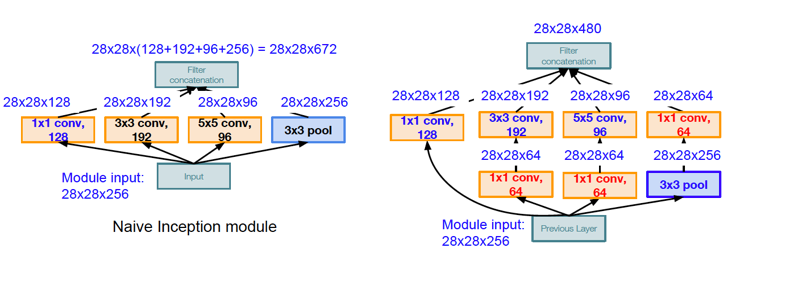
Figure 32
The InceptionNet design was based on the stacking of a base module callled the Inception Module (see Figure 32). As the LHS of the figure shows, the basic idea of the Inception module is to process the input data using multiple filters in parallel, before concatenating all their Activation Maps together and forming the input to the next stage (which we called Split/Transform/Merge earlier in this chapter). The Inception module uses four different types of convolutional engines: $1 \times 1$, $3 \times 3$, $5 \times 5$, and $3 \times 3$ with max-pooling. The smaller convolutions extract features at a finer level of detail, while the larger convolutions deal with features at a coarser level. However there is a problem associated with the architecture on the LHS: After the Activation Maps on all the four branches are concatenated, it results in 672 Activation Maps at the output of the module! As we add more modules, this will clearly result in an explosion in the number of Activation Maps, thus making the architecture infeasible. Another problem with the architecture is the extremely large number of numerical operations required to compute the activations.
The solution to these problems is shown on the RHS of Figure 32 and uses the concept of Bottlenecking with $1\times 1$ convolutions: We add three Activation Maps to the design that are generated using $1\times 1$ convolutions. The $1\times 1$ convolution in series with the Pooling layer reduces the number of Activation Maps in that branch from 256 to 64, which reduces the total number of Activation Maps at the output to 480. In addition two more $1\times 1$ convolutions are added to the $3\times 3$ and $5\times 5$ filter branches to compress the number of input Activation Maps to 64, before they are processed by the larger filters. This helps to reduce the number of numerical computations required from 854 million to 358 million.
The InceptionNet design aligns with the intuition that visual information should be processed at different scales and then aggregated so that the next stage can abstract features from different scales at the same time. The designers of the system also included a couple of extra output modules in the middle of the network (see Figure 31)), in order to amplify the error signal propagating towards the initial portion of the network, since they were concerned that the large number of layers in the network will cause the error signal to fade by the time it gets to the initial portion.
ResNet (2015)
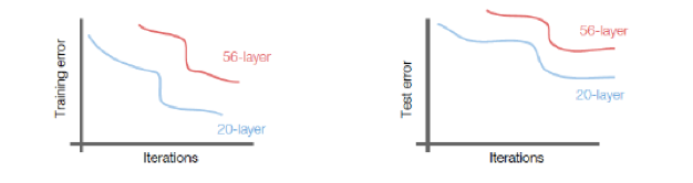
Figure 33
ResNets (short for Residual Neural Networks) were introduced by He, Zhang, Ren, Sun (2015), and this design won the ILSVRC 2015 competition by a wide margin, achieving a top 5 error error rate of 3.57%. ResNets have innaugurated the era of ultra-deep ConvNets, indeed the winning ResNet network came with 152 layers, an order of magnitude jump from the 22 layers in the previous year’s winner. The main architectural innovation in ResNets made such deep networks possible, and is based on the following insight: The number of layers in a ConvNet is constrained due to the fact that the error information propagating back during the backward phase of the Backprop algorithm, tends to get more and more diffused by the time it gets to the initial layers, due to multiplications with the weights and activations in the intervening layers. As a result the weights in the initial few layers are not modified in an optimal fashion during Gradient Descent. This effect is shown in Figure 33, which shows that both the Training and Test Error for a 56-layer network is higher when compared to that of a 20-layer network (which implies that the increase cannot be attributed to overfiting).
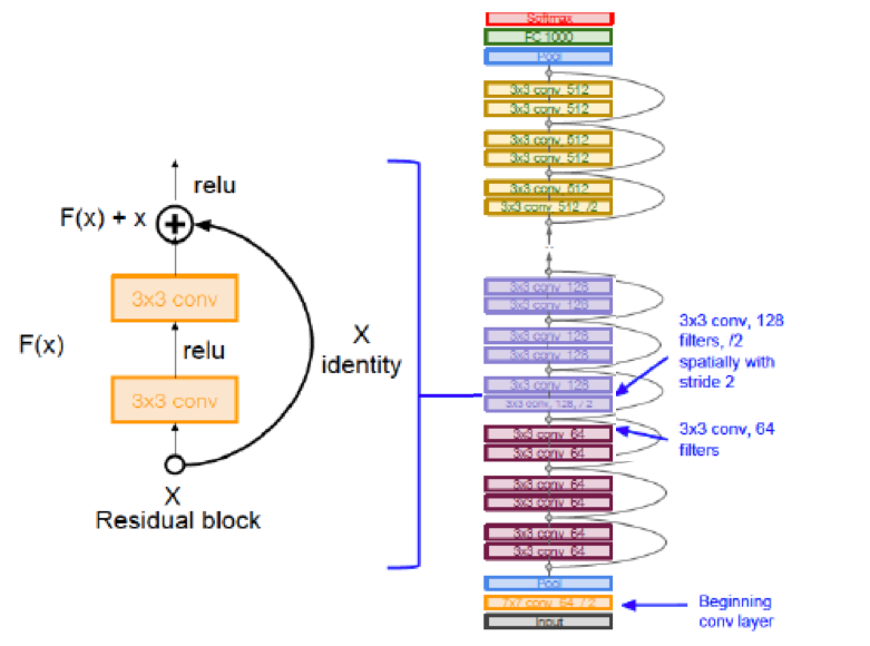
Figure 34
In order to overcome this problem, He, Zhang, Ren, Sun (2015) introduced a bypass link, as shown in LHS of Figure 34.
-
In the forward pass of Backprop, the bypass link enables the input signal to skip a few stacked Convolutional Layers, and then it is added to the output of these layers as shown. Note that the very first Convolutional Layer in the system is not bypassed. Hence one way to interpret this design is the following: The bypass enables the activation after the first convolutional layer to propagate all the way to the front of the network, while being modified by some delta (or residue) from each of the intervening bypassed layers. This design is based on the hypothesis that it is easier to optimize the residual mapping than to optimize the original, unreferenced mapping.
-
In the backward pass of Backprop, the bypass enables the error gradient information from the Output Layer of the network to propagate all the way to the first Convolutional Layer (with some modification from the gradients from the intervening layers). Hence all the layers in the network are able to access a strong signal from the error gradient information from the Output Layer, irrespective of the total number of layers in the network. This property enables ResNets to go Ultra-Deep without sacrificing performance.
Other interesting aspects of ResNets include the following:
-
The system makes extensive use of Batch Normalization, see Section BatchNormalization, which is implemented at the end of every layer.
-
It uses a relatively large Learning Rate of 0.1 (Section LearningRateSelection), which is divided by 10 whenever the validation error plateaus during training. Such a large rate is made possible due to the use of Batch Normalization.
-
The system does not make use of Dropout normalization (Section DropoutRegularization). It is theorized that Dropout is not needed in the presence of Batch Normalization.
-
The system does not make use of Dense layers at the end of the network.
ResNets are still among the best performing ConvNets and are used by default in practical cases.
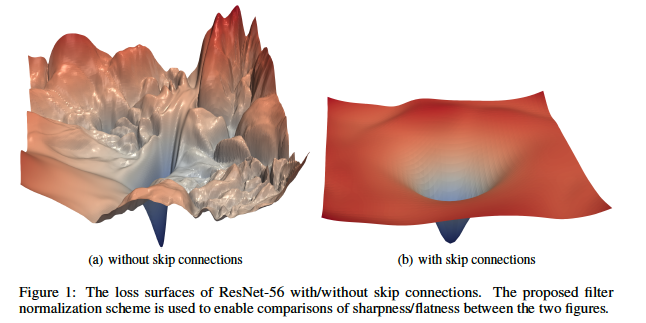
Figure 35
There has been some recent work by Li, Xu et.al. which beautifully shows the beneficial effect of adding Residual Connections. They achieved this by coming up with a new way to visualize Loss Surfaces for a Neural Network, examples of which are shown in Figures 35 and 36. Part (a) of Figure 35 shows the Loss Surface for a 56 layer ResNet without any Residual Connections, while Part (b) shows the Loss Surface for the same network after the addition of Residual Connections. As can be seen, the Loss Surface has become much more smooth and convex in shape, which makes it easier to run the SGD algorithm on it. In contrast, the chaotic shape of the Loss Surface without residual connections makes it very easy for the SGD algorithm to get caught in local minimums. There is a single large minima in the Loss Surface without Residual Connections, however for the SGD to get to it, it needs to initialized properly. This also implies, that without Residual Connections, the effectiveness of SGD is highly dependent on the initialization values.
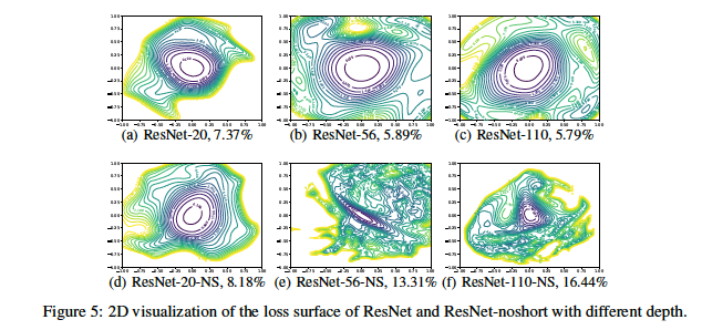
Figure 36
The contour plots in Figure 36 shows the effect of the network depth on the Loss Surface, both with and without Residual Connections. We observe the following:
- Networks with a smaller number of layers, such as the 20 layer ResNet on the LHS, exhibit fairly well behaved Loss Surfaces, even in the absence of Residual Connections. Hence Residual Connections are not essential for smaller networks.
- Networks with a larger number of layers on the other hand, start to exhibit chaotic non-convex behavior in their Loss Surface in the absence of Residual Connections.
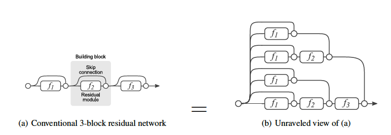
Figure 37
Another very interesting perspective on why Residual Connections are so effective was provided by Veit, Wilbur, Belongie. Instead of looking at the backward flow of gradients, the focused on the forward path of ResNet, and noted the following:
-
In a network with no Residual Connections, there exists only a single forward path and all data flows along it. However in a network with n Residual Connections, there exist $2^n$ forward paths. This is illustrated in Figure 37 for the case $n=3$. The 8 separate forward paths that exist in this network are shown in Part (b) of this figure. As a result, the network decisions are effectively made by all of these 8 forward paths, that are operating parallel. This is very much like what is done in the Ensemble method, in which multiple models operate in parallel to improve model accuracy.
-
They furthermore showed that gradient flow in the backwards direction is dominated by a few shorter paths. This is illustrated in Figure 38 which has results for a network with 54 Residual Connections. Part (a) of this figure shows the distribution of the path lengths in this network, while Part (b) plots the gradient magnitudes. They further multiplied the gradient magnitudes with the number of pathlengths for a particular path, and and obtained the graph in Part (c). As can be seen the majority of the gradients are contributed by path lengths of 5 to 17, while the higher path lengths contribute no gradient at all. Fom this they concluded that in very deep networks with hundreds of layers, Residual Connections avoid the vanishing gradient problem by introducing short paths which can carry the gradient throughout the extent of these networks.
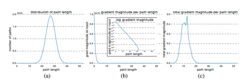
Figure 38
Beyond ResNets: ResNext and DenseNet
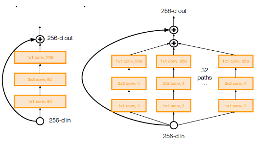
Figure 39
The base ResNet design can be improved by applying the techniques discussed earlier in this chapter, two of which are shown in Figure 39:
- The Left Hand Side of the figure shows the application of Bottlenecing using $1\times 1$ filter, which reduces the number of parameters and computation by almost a factor of 3
- The Right Hand Side of the figure shows the application of Split/Transform/Merge to ResNet, which results in a network called ResNext.
A 101-layer ResNeXt was able to achieve better accuracy than a 200-later ResNet even though it has only 50% of the parameters. ResNeXt was submitted to the ILSVRC 2016 classification task, in which it secured second place.
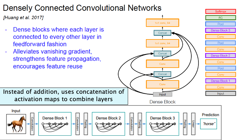
Figure 40
DenseNets are built from modules called Dense Blocks as shown in the lower part of Figure 40. Within each Dense Block, the Activation Maps of all preceding layers are used as inputs into the next convolutional layer, and its own Activation Maps are used as inputs into all subsequent layers. In contrast to ResNets, DenseNets don’t combine features through summation before they are passed into a layer; instead, they combine features by concatenating them. DenseNets use smaller number of Activations Maps per layer (only 12) compared to ResNets, which results in a decrease in the number of parameters. It is likely that the concatenation of layers makes up for this reduction. The Table ConvNetPerformance shows that DenseNets are able to outperform ResNets with a smaller model size.
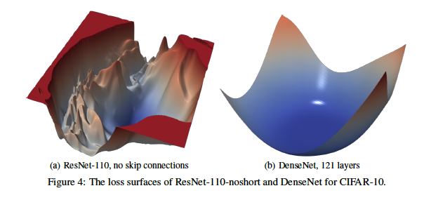
Figure 41
The DenseNet architecture is quite effective in making the shape of the Loss Function surface more convex and hence easier to optimize, as shown in Part(b) of the above figure (taken from Li, Xu et. al.
Xception
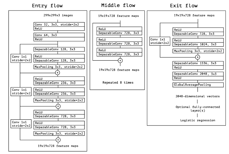
Figure 42
The Xception architecture replaces the regular Convolution operation by Depthwise Separable convolutiion in all its layers except for the first two. It has 36 convolutional layers forming the feature extraction base of the network. These convolutional layers are structured into 14 modules, all of which have linear residual connections around them, except for the first and last modules.
The Xception network has performance that is comparable with the Google InceptionNet, but with a smaller parameter count.
MobileNet
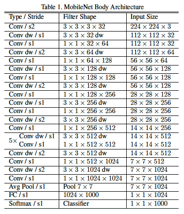
Figure 43
MobileNet belongs to the same category of architectures as Xception, since it uses Depthwise Separable Convolutions to bring down the parameter count. The motivation behind MobileNet was to come up with a design that could be deployed in real world applications such as robotics, self-driving car and augmented reality. These involve tasks need to be carried out in a timely fashion on a computationally limited platform with small low latency models.
The MobileNet architecture is defined in Figure 43 (note that a filter shape of $1\times\times 1\times 128\times 256$ denotes a $1\times 1$ filter with 128 Activation Maps in the input layer and 256 Activation Maps in the output layer). All layers are followed by a batchnorm and ReLU nonlinearity with the exception of the final fully connected layer which has no nonlinearity and feeds into a softmax layer for classification. A final average pooling reduces the spatial resolution to 1 before the fully connected layer. Counting depthwise and pointwise convolutions as separate layers, MobileNet has 28 layers. As the Table in Figure 26 shows, this results in a model with the smallest number of parameters, with some decrease in accuracy.
Visualizing ConvNets
ConvNets seem to work very well and constitute a significant advance in neural network architecture. However their decision making process proceeds through complex non-linear computations that are opaque to humans. In order to gain more confidence in the output of these networks, it would be nice if we can get some insights into how they go about doing their job. The field of ConvNet Visualization attemtps to do this in various ways that are described in this section. In particular we will describe the following techniques:
- Visualizing the last layer in the Feature Space: The Last Layer before the classification step represents the results of all the transformations on the original image, and hence visualizing its co-ordinates gives insights into the ConvNets’s operation.
- Visualizing Local Filters: Using the template matching interpretation of image recognition, the shape of local filters can tell us the kind of objects the network is looking for.
- Identifying Maximally Activating Patches in Images: This technique solves the following problem: Given a neuron that gets activated by an image, identify the portion of the image that it is reacting to.
- Generating Images that Maximize Neuron Activations: This is the process of running the ConvNet backwards to generate images that maximize the activation at a chosen neuron.
- Generating Images from Feature Vectors: This also involves running the ConvNet backwards, to generate images whose Feature Vectors match those from a sample image.
Visualizing the Proximity Property of Feature Space Representations
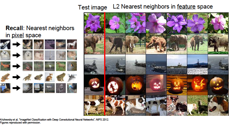
Figure 44
We have emphasized the fact that Deep Learning Networks transform the representation of images from RGB pixels to a feature space representation that also carries semantic information, such that images that are in the same category tend to have representations that cluster together in feature space. This property can be verified by examining the L2 nearest neighbors for an image, as shown in the RHS of Figure 44. This figure shows the sample image in the first column on the left side of the figure, while the images in each row correspond to images whose feature space L2 distance is closest to the sample image in that row. The feature space representation is obtained as the activations of the FC2 Fully Connected layer in AlexNet. We note the following:
- Images whose pixel values are very different are nevertheless close to each other in feature space, thus verifying the semantic clustering property of DLNs.
- On the other hand, relying on L2 nearest neighbors in pixel space is not a reliable way of clustering images, since it can result in images that are in different categories, as shown on the LHS of Figure 44.
Visualizing Local Filters
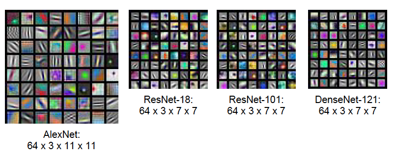
Figure 45
Consider a ConvNet, such as AlexNet, with 64 Activation Maps in the first Convolutional Layer which are generated using 64 local filters of size $11\times 11$. Each of these filters can be visualized by using the filter values to generate a $3\times 11\times 11$ color image, and this is shown in Figure 45 for AlexNet as well as for a few other types of ConvNets. Using the template matching interpretation of local filtering, it follows that first Hidden Layer filters in all these networks are mostly looking for simple patterns such as straight edges in various orientations. Hubel and Wiesel had discovered that the visual system in animals has a similar property, in that the first layer of neurons in the visual cortex is sensitive to the presence of edges in the image falling on the retina.
Unfortunately it is not possible to as readily visualize filters in the deeper layers of the network, due to the fact that they possess a depth of more than 3 and hence cannot be converted into a color image. Hence in order to understand what is happening in the deeper layers of the network, we rely on techniques described in the following sub-sections.
Visualizing Activation Maps
Unlike Convolutional Filters, Activation Maps can be visualized for all layers of a network, since each of them can be considered to be a grayscale image. This exercise was carried out in Section 5.4.1 of the book Deep Learning with Python and the results are summarized for the cat image shown below.
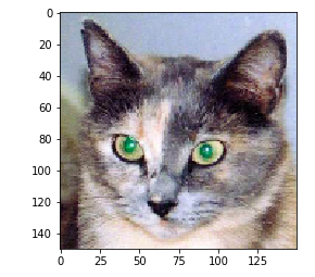
Figure 46
Figure 47 graphs some of the Activation Maps in Convolutional Layer 1 and Layer 8 of an 8 layer ConvNet, for the input image in Figure 46. We note tha following:
- Recall that the Activations Maps in Layer 1 act as detectors of simple shapes such as edges of various types. The Activation Maps figures in Layer 1 bear this out, since most of them outline the shape of the cat which is where the edges occur.
- An examination of the Layer 8 Activation Maps on the other hand shows that they have very little resemblance to the original image. In most Activation Maps a few of the neurons show higher activation than the others (these are coded in yellow). These are responding to some higher level aspect of the input image, but we can’t tell what that is from the Activation Maps figures alone. Thus higher level activations carry more and more information about the presence or absence of certain complex patterns in the input image, rather than the shape of the image itself. If a neuron has zero activation then it means that the pattern it is looking for is not present in the input image.
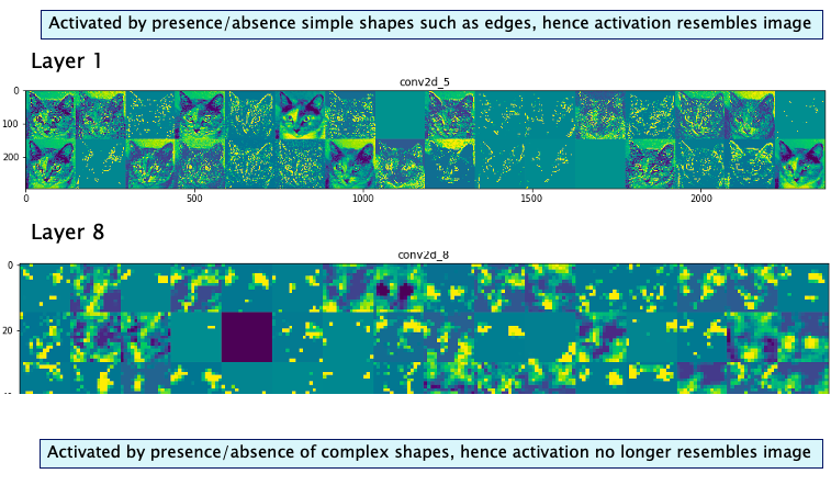
Figure 47
Identifying Maximally Activating Patches in Images
In the previous section we surmised that the neurons in the higher convolutional layers are activated by more complex patterns in the input image while the lower layers are activated by simpler paterns. This intuition can be verified by using the concept of Maximally Activating Patches, which are defined as follows: Pick any neuron in a ConvNet, it can be one of the logit nodes whose activation is equal to the class-score of the corresponding category, or it can be a neuron in one of the Activation Maps within a convolutional layer. Assuming that the input image is such that it results in a high activation value at the chosen node, i.e., the neuron reponds positively to some pattern that it detects in the image. Then the Maximally Activating Patch is defined to be the localized portion of the image that the neuron is responding to.
Maximally Activating Patches are identified by running the ConvNet backwards, which is actually a very important notion. Though originally proposed as a way to identify Maximally Activating Patches, the backwards operation has since been extended to tasks that involve generating new images from a trained ConvNet.
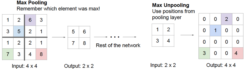
Figure 48: Backwards_Propagation_through_MaxPooling
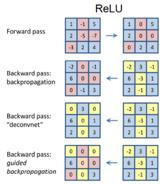
Figure 49: Backwards_Propagation_through_ReLU
There are two main techniques that are used to run a ConvNet backwards:
- DeConvNet
- Guided Backpropagation
Both these techniques use the same computations for going backwards through Convolutional and Pooling layers, but differ in the way they pass through ReLU non-linearities. These operations are described next:
-
Backwards through Convolutional Layers: This operation is the same as that carried out by backpropagating gradients in the Backprop algorithm, and involves multiplication by the transpose of the Convolutional Filter.
-
Backwards through Pooling Layers: This operation is referred to as “switching” and proceeds as follows: Carry out a forward pass through the network, and keep record of the positions at which the maximum activation in max-pooling occurs (see Figure 48). In the backward pass, the incoming activation is placed in the “maximum activation” spot, while all the activations are set to zero.
-
Backwards through ReLU Non-Linearities: As shown in Figure 49, there are multiple ways in which a ConvNet can be run backwards through ReLU non-linearities:
- The top row of the figure shows a Forward Pass through a ReLU non-linearity. It shows the negative pre-activations on the LHS being reset to zero in order to generate activation numbers on the RHS of the figure.
- The second row in the figure shows a backward pass through a ReLU for gradients using traditional Backprop: Recall that the ReLU non-linearity acts as a switch for the gradients during Backprop, so that the negative pre-activations (in the LHS of the top row) cause the gradients in the corresponding positions to go to zero.
- The third row in the figure shows the ReLU backward pass used in DeConvNets. When going backwards through a ReLU non-linearity, all negative values are set to zero, as shown. In contrast to Backprop and Guided Backprop (see below), the numbers flowing back during the DeConvNet operation should not be thought of as gradients, they should be regarded as “activations”” that are propagating backwards.
- The fourth row in the figure shows a backward pass for gradients used in Guided Backpropagation. When passing backwards through ReLU non-linearity, the negative gradients are set to zero, in addition to the gradients for whom the corresponding input activation is negative. Hence the Guided Backpropagation ReLU backpropagation rule combines the rules for Regular Backpropagation + DeConvNet Backpropagation.
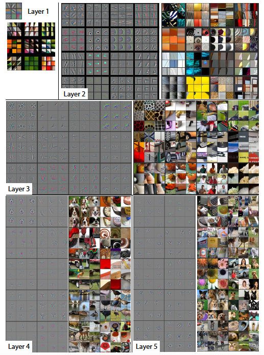
Figure 50
We now describe the application of DeConvNets to the problem of finding out the portion of an image that an individual neuron is responding to (also called the Maximally Activating Patch):
- Start with a fully trained ConvNet model (such as on ImageNet) and present it with an input image. Do a forward pass through the model and compute all the activations.
- To examine a given activation, say $a$, (which has been activated by the image), set all the other activations in its Activation Map to zero (as well as the activations of the other Activation Maps in its layer) and pass this as input to the DeConvNet network.
- Propagate the signal backwards using the DeConvNet propagation rules described above, until the pixel space is reached. This results in the computation of ${\partial a\over{\partial x_{ijk}}}$ for all the pixels $x_{ijk}$ in the image.
The reconstructed image obtained by plotting ${\partial a\over{\partial x_{ijk}}}$ for AlexNet (trained on ImageNet) is shown for activations in Layers 1 to 5 in Figure 50. For each layer, the images on the LHS show the actual reconstruction, while the corresponding images on the RHS are portions of the input image that were identified by the reconstruction. Note that the nine largest activations were chosen in each of the Activation Maps. We can draw the following conclusions from these images:
- The reconstructed image resembles a small piece of the original input image, with the shapes in the input weighted according to their contribution to the neuron whose activation was propagated back.
- All the neurons in a single Activation Map seem to get activated by similar shapes, and this shape varies with the Activation Map. This property is stronger in the higher layers.
- As we go up the layers, the activations get triggered by more and more complex shapes and objects.
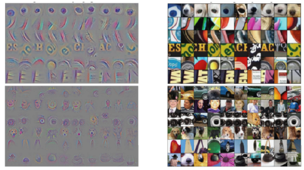
Figure 51
A similar procedure can be carried out using the Guided Backpropagation procedure, and the results for Convolutional Layers 6 and 9 for AlexNet are shown in Figure 51 (with the reconstructed image on the LHS and the corresponding patch from the actual image on the RHS). This figure shows that the reconstructed image quality is better with Guided Backpropagation.
Generating Images
Generating images using ConvNets is one of the most exciting areas in Deep Learning, and as a field is still undergoing rapid development. There are several ways in which ConvNets are being used to generate images, and in this section we explore a few of them:
- Generating images that maximally activate a neuron
- Images generated using Google’s Deep Dream algorithm
- Generating images by Feature Inversion
One of the realizations that we have to come based the image generation work, is that a trained Neural Network contains a lot of detailed information about the objects as well as other parts of the image in its training dataset, which is enough to actually generate images of these objects. Previously it was thought that Supervised Learning models incorporated only very basic high level information about objects, which was just sufficient to be able to recognize them. It is also possible to generate images using ConvNets with the help of Unsupervised Learning techniques such as Generative Adversarial Networks (GANs) and PixelCNN, but these are not covered in this chapter.
Generating Images that Maximally Activate a Neuron
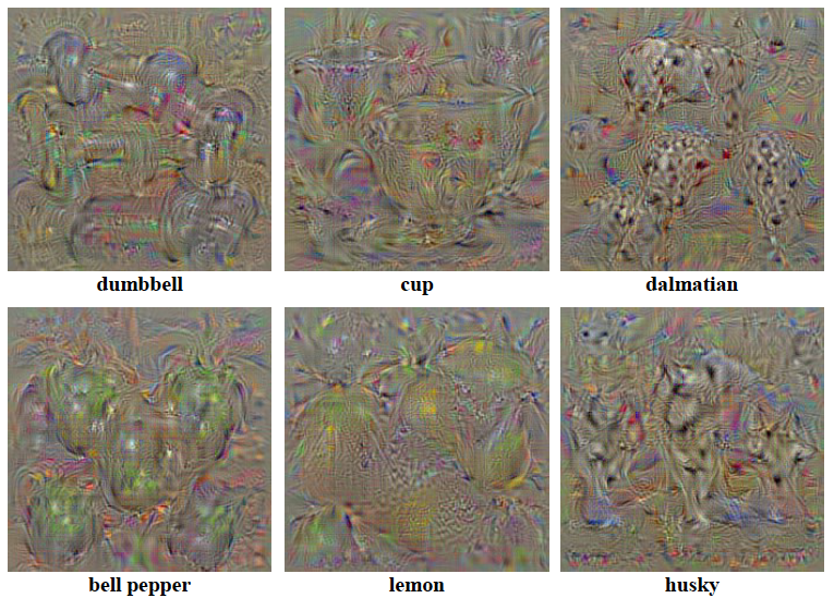
Figure 52
Start with a fully trained ConvNet, and keep its weights fixed during this procedure. Solve the following maximization problem:
Find an image $I$ that maximizes the following Loss Function
\[\mathcal L = S_c(I) - \lambda ||I||^2_2\]In this equation, the $S_c(I)$ is the Score Function for the $c^{th}$ class, and is computed by doing a forward pass through the ConvNet. The second term is added for doing Regularization, with $\lambda$ as the Regularization Parameter. It had been experimentally observed that without the Regularization Term, the optimization procedure results in an image that looks like white noise.
The following algorithm is used to do the optimization:
- Start with a trained ConvNet (trained on zero centered image data) and fix the value of its weights. Initialize the image pixel values $x_{ijk}$ to zero.
- Repeat Steps 3 to 5 until a Stopping Condition is satisfied
- Do a forward pass through the network and compute the Score Function $S_c(I)$ and Loss Function $\mathcal L$.
- Starting with the gradient $\frac{\partial\mathcal L}{\partial S_c}$, use the Backprop algorithm to compute the gradients $\frac{\partial\mathcal L}{\partial x_{ijk}}$ of the Loss Function with respect to each of the image pixel values
- Change the pixel values using the following iteration:
- Add the training set mean image to the final pixel values to obtain the final image.
Figure 52 shows the results of applying this algorithm to a ConvNet trained on the ImageNet dataset. The reader will notice the objects belonging to the category whose Score Function is being maximized, emerging at multiple places in each image, but with colors that are different than the natural coloration of the object. The reason for this is that the neurons in the later layers of the network, and especially the classification neurons, incorporate more invariance in their object recognition. Hence they recognize an object irrespective of its color or location in the image and this invariance property gets reflected in the generate images. It is possible to generate images that are more pleasing to the eye, and some of these are shown in Figure 53. These images were generated by making the following changes to the algorithm described above:
- Incorporation of the Total Variation (TV), Gaussian Blur and Jitter regularizers into the Loss Function
- Initialize the image by using the average of the images in that category from the test dataset (if an image has multiple facets, then averaging is done over one of the facets)
- Use of Gaussian Blur regularization results in a blurry, but single and centered object. The optimization then proceeds by updating the center pixels more than the edge pixels to produce a final image that is sharp and is centrally located.
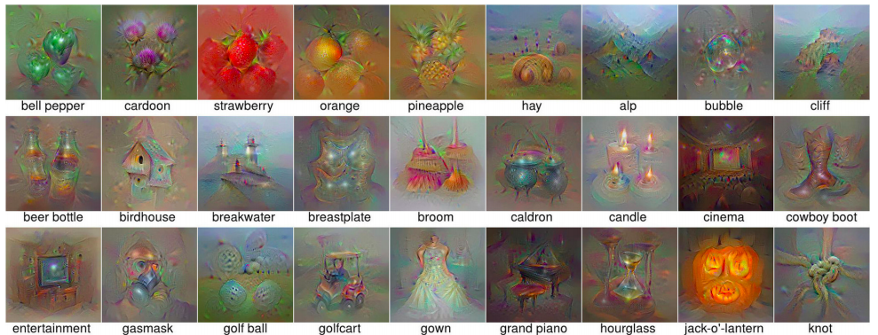
Figure 53
Adversarial Images
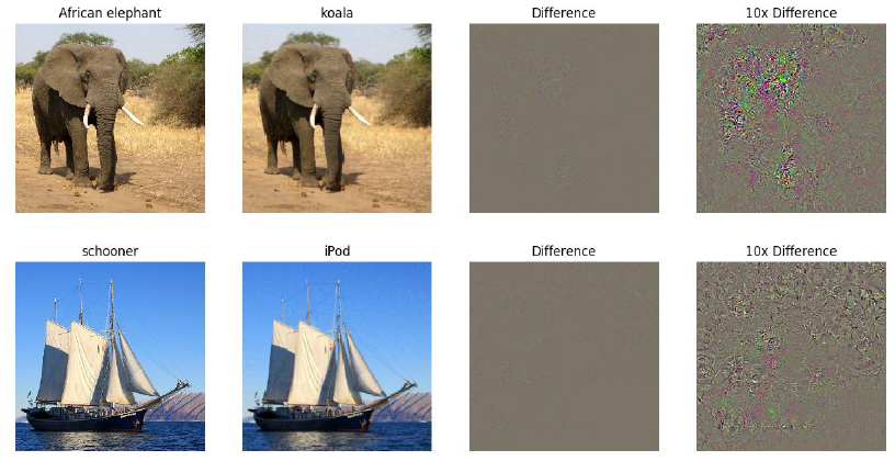
Figure 54
It has been shown that ConvNets can be fooled into mis-classifying images. A couple of examples of this are shown in Figure 54: In the top row the first image is classified correctly as an elephant. Then this image is modified by changing some the pixels (which are shown in the last two columns), which results in the second image. These changes are not perceptible to the human eye since the second image also looks like an elephant, however when sent through a ConvNet, the system classifies it as a koala. A similar process applied to the boat in the bottom row, results in its mis-classification as an iPod. These images, which fool the ConvNet into mis-classifying them, are known as Adversarial Images.
Adversarial images can be easily created by making a slight modification to the algorithm that was presented in the prior section for generate images that maximally activate neurons. The only changes needed are the following:
- Instead of initializing the input image with zeroes, we initialize it with the image whose adversarial example we wish to generate.
- Choose the neuron whose activation is to be maximized, as the classification node for the adversarial image class.
We then run the maximization algorithm, and after a few iterations, the system will mis-classify the input image even though it does not appear to have changed.
Adversarial Images are an active research topic, since they constitute a significant security loophole that can perhaps be exploited.
Generating Images Using Google Deap Dream
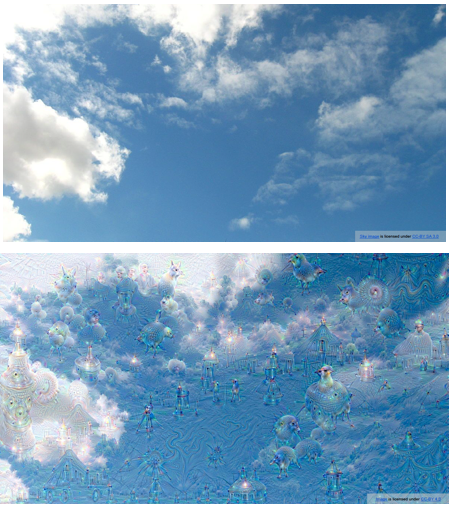
Figure 55
Google Deep Dream uses the following algorithm to generate images:
- Start with a trained ConvNet (trained on zero centered image data) and fix the value of its weights. Initialize the image pixel values $x_{ijk}$ to some random image from the test dataset. In the example in Figure 55, the initial image was chosen to be that of clouds, shown on top part of the figure.
- Repeat Steps 3 to 6 until a Stopping Condition is satisfied
- Do a forward pass through the network and compute the activations at all the nodes, up until a chosen layer.
- Set the gradients at each node of the chosen layer equal to the activation at that node, i.e.,
- Using the Backprop algorithm compute the gradients $\frac{\partial\mathcal L}{\partial x_{ijk}}$ of the Loss Function with respect to each of the image pixel values
- Change the pixel values using the following iteration:
- Add the training set mean image to the final pixel values to obtain the final image.
In the example in Figure 55, the ConvNet was trained using ImageNet. The top part of the figure show the input image, and after a number of iterations, the original image changes to the one shown in the bottom of figure. The Deep Dream algorithm tends to amplify random features in the original image, until they start to resemble objects that were part of the network’s original training set. Note that setting the gradient equal to the activation is equivalent to using the following Loss Function:
\[\mathcal L = {1\over 2}\sum_i z_i^2\]where the sum is over all the activations in a given layer.
Generating Images Using Feature Inversion
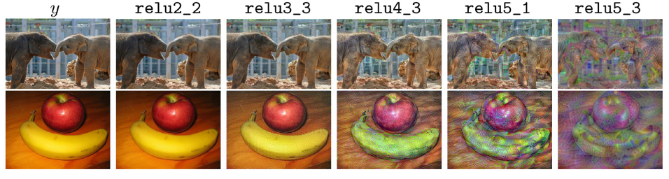
Figure 56
The image generation techniques that we have described so far, do their work by iteratively creating images that maximally activate a neuron. There is another technique, which instead of trying to maximize neuron activations, instead works by generating images whose Feature Vector is specified in advance. In order to do so, the following Loss Function is used:
\[\mathcal L = ||\Phi(X) - \Phi_0||^2 + \lambda_\alpha \mathcal R_\alpha(X) + \lambda_{V^\beta}\mathcal R_{V^\beta}(X)\]where the Regularisers $\mathcal R_{\alpha}$ and $\mathcal R_{V^\beta}$ are set to
\[\mathcal R_\alpha(X) = ||X||^\alpha_\alpha,\ \ {\mbox and}\ \ \mathcal R_{V^\beta}(X) = \sum_{i,j} ((x_{i,j+1} - x_{ij})^2 + (x_{i+1,j} - x_{ij})^2)^{\beta\over 2}\]In these equations $\Phi_0$ is the Feature Vector from the test image that the algorithm is trying to match, while $\Phi(X)$ is the Feature Vector from the current iteration of the generated image. Note that the addition of the Regularisers $\mathcal R_{\alpha}$ and $\mathcal R_{V^\beta}$ is critical to generating “good” images. In their absence, the algorithm will generate images whose Feature Vector minimizes the Loss Function, but which look like noise to the human eye.
The algorithm is as follows:
- Start with a trained ConvNet (trained on zero centered image data) and fix the value of its weights. Initialize the image pixel $x_{ijk}$ to some random values. The example in Figure 56 shows two different test images in the leftmost image in each row.
- Repeat Steps 3 to 5 until a Stopping Condition is satisfied
- Do a forward pass through the network and compute the activations at all the nodes, up until a chosen layer.
- Compute the gradients $\frac{\partial\mathcal L}{\partial\Phi}$ at each node of the chosen layer and use the Backprop algorithm compute the gradients $\frac{\partial\mathcal L}{\partial x_{ijk}}$ of the Loss Function with respect to each of the image pixel values
- Change the pixel values using the following iteration:
- Add the training set mean image to the final pixel values to obtain the final image.
The images generated by running this algorithm are shown in Figure 56. The notation relu2_2 is used to denote the images generated by matching feature vectors in the second layer and so on. As the figure shows, the generated images in the first few layers closely match the original test image, which implies that the ConvNet is able to store fine level details regarding the test image with a high level of fidelity. As we go to the higher layers, the image content and the overall spatial structure are preserved, but the color, texture and exact shape are not.
This procedure shows that the activations at a particular layer can be used to ‘encode’ an image. Hence instead of transmitting the original image, we instead send the activations from one of the layers. At the receiving end, we use these activations plus our knowledge of the pre-trained model which generated the activations to ‘de-code’ the image back.
Other Image Processing Tasks
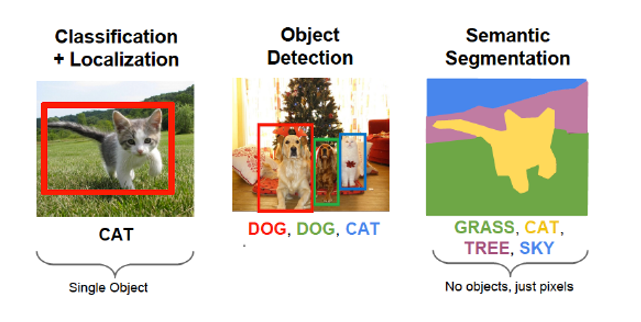
Figure 57
In addition to Classification, ConvNets are also used to solve several important Image Processing tasks. We discuss the following in this section:
- Object Localization: This involves having the model put a box around the object, in addition to classifying it.
- Semantic Segmentation: This is defined as the process of classifying each and every pixel in an image, into a fixed number of categories.
- Object Detection: Object Localization is restricted to boxing a single object (or a fixed number of them). If the number of objects to be boxed and identified is variable and not known in advance, then the problem becomes that of Detection.
Examples of thesee three types of image processing are shown in Figure 57.
Object Localization
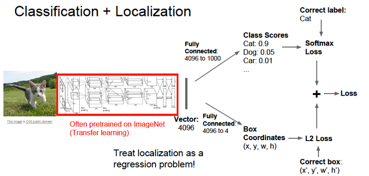
Figure 58
The Classification + Localization problem can be solved by training a model to predict the co-ordinates of the 4 corners of the bounding box, in addition to classifying the object. In order to do so, the modeler has to create a training dataset in which the label identifies the co-ordinates of the box. Once this done, the training can proceed using the type of model shown in Figure 58. It shows a so-called ‘two-headed’ Convnet, with the body consisting of the convolutional base. The output from the base is routed to Dense Networks, with Network One connected to the logits for classifying the object (using the Softmax Loss) and Network Two connected to a Regression Layer that predicts the box co-ordinates (using the Mean Square Error or L2 Loss). The Backprop algorithm is then run on the combined loss. As the figure shows, Transfer Learning can be used for this problem with a pre-trained Convolutional Base, as long as the objects to be classified are not too different than the ImageNet dataset.
Semantic Segmentation
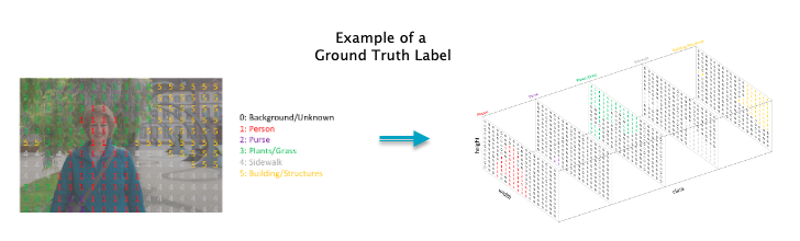
Figure 59
Semantic Segmentation is the problem of classifying each and every pixel in an image into a fixed number of categories. It has a number of important application, for example it can be used by the vision system in a self-driving car to differentiate the road, pedestrians, trees etc. In order to train a model to do Semantic Segmentation we need an appropriate training dataset in which every pixel is labeled, an example of which is shown in Figure 59. In this example all the pixels are given one of 5 labels, and this information is captured using multiple Label Maps as shown.
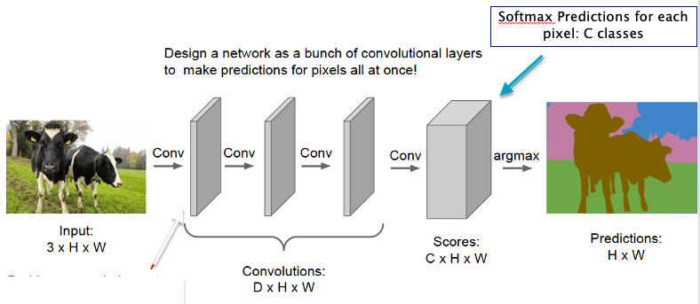
Figure 60
The objective of the Semantic Segmentation model is to predict a Label Map for the input image, and this can be done using ConvNets as shown in Figure 60. The input image is sent through multiple convolutional layers, and the final prediction is in the form of a 3D tensor with C layers (corresponding to C pixel categories). For the $c^{th}$ layer, the model predicts a total of $H\times W$ binary valued probabilities of the pixels belonging to the $c^{th}$ category. The final prediction for a pixel location is the category that has the maximum probability value.
Object Detection
Object Detection is a challenging problem since the number of objects in the image is not known in advance. An initial attack on this problem led to an algorithm called R-CNN (stands for Region based CNN) in which a ConvNet model was used to detect images over several region candidates in the image (these region candidates were generated seprately by a non-ML algorithm). This did work but was very expensive, since each image required several forward passes through the model. An algorithm called YOLO (for ‘You only Look Once’) was proposed subsequently, which is much more efficient since it can do its job with just a single forward pass. This makes it suitable for real time detection tasks, such as detecting objects in a video clip.
The YOLO algorithm takes the following steps to do detection (see Figure 61):
- The image is divided into a grid of size $S\times S$ as shown in the LHS of the figure
- For each grid cell, the model predicts $B$ Bounding Boxes as potential candidates for object detection, for a total of $BS^2$ Bounding Boxes. This is shown in the top half of the figure.
- The model predicts a confidence score for each bounding box, which is defined as $P(Object)*IOU^{truth}_{predict}$. These confidence scores reflect how confident the model is that the box contains an object and also how accurate it thinks the box is that it predicts.
- Lastly, for each grid cell, the model predicts the softmax probability vector of it containing one of the $C$ objects $P(Class_i\vert Object), 1\le i\le C$, i.e. the conditional probability of class $i$ given that the grid cell contains an object. This is illustrated in the bottom part of the figure.
The model’s final prediction is obtained by doing the following computation:
\[Pr(Class_i|Object) ∗ Pr(Object) ∗ IOU^{truth}_{pred} = Pr(Class_i) ∗ IOU^{truth}_{pred}\]This computation gives us class-specific confidence scores for each box. These scores encode both the probability of that class appearing in the box and how well the predicted box fits the object.
Figure 61
The YOLO Model is shown in Figure 62, for the case $S = 7, B = 2$ and $C = 20$. This system models detection as a Regression problem. Note that the final predictions are encoded as a $S\times S\times (5B+C)$ tensor since the model predicts $5B+C$ numbers for each grid cell: $x,y,w,h$ and $confidence$, where the $(x, y)$ coordinates represent the center of the box relative to the bounds of the grid cell. The width and height are predicted relative to the whole image and the confidence prediction represents the IOU between the predicted box and any ground truth box.
Figure 62